Expected output¶

InStrain produces a variety of output in the IS folder depending on which operations are run. Generally, output that is meant for human eyes to be easily interpretable is located in the output folder.

inStrain profile¶

A typical run of inStrain will yield the following files in the output folder:

scaffold_info.tsv¶

This gives basic information about the scaffolds in your sample at the highest allowed level of read identity.

scaffold_info.tsv¶
scaffold	length	coverage	breadth	nucl_diversity	coverage_median	coverage_std	coverage_SEM	breadth_minCov	breadth_expected	nucl_diversity_median	nucl_diversity_rarefied	nucl_diversity_rarefied_median	breadth_rarefied	conANI_reference	popANI_reference	SNS_count	SNV_count	divergent_site_count	consensus_divergent_sites	population_divergent_sites
N5_271_010G1_scaffold_100	1148	1.89808362369338	0.9764808362369338	0.0	2	1.0372318863390368	0.030626273060932862	0.018292682926829267	0.8128805020451009	0.0			0.0	1.0	1.0	0	0	0	0	0
N5_271_010G1_scaffold_102	1144	2.388986013986014	0.9956293706293706	0.003678160837326971	2	1.3042095721915248	0.038576628450898466	0.07604895104895107	0.8786983245100435	0.0			0.0	1.0	1.0	0	0	0	0	0
N5_271_010G1_scaffold_101	1148	1.7439024390243902	0.9599303135888502		2	0.8728918441975071	0.025773816178570358	0.0	0.7855901382035807				0.0	0.0	0.0	0	00	0	0
N5_271_010G1_scaffold_103	1142	2.039404553415061	0.9938704028021016	0.0	2	1.1288397384374758	0.03341869350286944	0.04028021015

scaffold: The name of the scaffold in the input .fasta file
length: Full length of the scaffold in the input .fasta file
coverage: The average depth of coverage on the scaffold. If half the bases in a scaffold have 5 reads on them, and the other half have 10 reads, the coverage of the scaffold will be 7.5
breadth: The percentage of bases in the scaffold that are covered by at least a single read. A breadth of 1 means that all bases in the scaffold have at least one read covering them
nucl_diversity: The mean nucleotide diversity of all bases in the scaffold that have a nucleotide diversity value calculated. So if only 1 base on the scaffold meets the minimum coverage to calculate nucleotide diversity, the nucl_diversity of the scaffold will be the nucleotide diversity of that base. Will be blank if no positions have a base over the minimum coverage.
coverage_median: The median depth of coverage value of all bases in the scaffold, included bases with 0 coverage
coverage_std: The standard deviation of all coverage values
coverage_SEM: The standard error of the mean of all coverage values (calculated using scipy.stats.sem)
breadth_minCov: The percentage of bases in the scaffold that have at least min_cov coverage (e.g. the percentage of bases that have a nucl_diversity value and meet the minimum sequencing depth to call SNVs)
breadth_expected: expected breadth; this tells you the breadth that you should expect if reads are evenly distributed along the genome, given the reported coverage value. Based on the function breadth = -1.000 * e^(0.883 * coverage) + 1.000. This is useful to establish whether or not the scaffold is actually in the reads, or just a fraction of the scaffold. If your coverage is 10x, the expected breadth will be ~1. If your actual breadth is significantly lower then the expected breadth, this means that reads are mapping only to a specific region of your scaffold (transposon, prophage, etc.)
nucl_diversity_median: The median nucleotide diversity value of all bases in the scaffold that have a nucleotide diversity value calculated
nucl_diversity_rarefied: The average nucleotide diversity among positions that have at least --rarefied_coverage (50x by default). These values are also calculated by randomly subsetting the reads at that position to --rarefied_coverage reads
nucl_diversity_rarefied_median: The median rarefied nucleotide diversity (similar to that described above)
breadth_rarefied: The percentage of bases in a scaffold that have at least --rarefied_coverage
conANI_reference: The conANI between the reads and the reference genome
popANI_reference: The popANI between the reads and the reference genome
SNS_count: The total number of SNSs called on this scaffold
SNV_count: The total number of SNVs called on this scaffold
divergent_site_count: The total number of divergent sites called on this scaffold
consensus_divergent_sites: The total number of divergent sites in which the reads have a different consensus allele than the reference genome. These count as “differences” in the conANI_reference calculation, and breadth_minCov * length counts as the denominator.
population_divergent_sites: The total number of divergent sites in which the reads do not have the reference genome base as any allele at all (major or minor). These count as “differences” in the popANI_reference calculation, and breadth_minCov * length counts as the denominator.

mapping_info.tsv¶

This provides an overview of the number of reads that map to each scaffold, and some basic metrics about their quality. The header line (starting with #; not shown in the table below) describes the parameters that were used to filter the reads

mapping_info.tsv¶
scaffold	pass_pairing_filter	filtered_pairs	median_insert	mean_PID	pass_min_insert	unfiltered_reads	unfiltered_pairs	pass_min_read_ani	filtered_priority_reads	unfiltered_singletons	mean_insert_distance	pass_min_mapq	mean_mistmaches	mean_mapq_score	unfiltered_priority_reads	pass_max_insert	filtered_singletons	mean_pair_length
all_scaffolds	22886	9435	318.75998426985933	0.942328296264744	22804.0	71399	22886	9499.0	0	25627	322.1849602376999	22886.0	14.325963471117715	17.16896792799091	0	22828.0	0	255.52
N5_271_010G1_scaffold_1	432	346	373.0	0.9719013034762376	432.0	959	432	346.0	0	95	373.72222222222223	432.0	7.643518518518517	33.030092592592595	0	432.0	0	274.7106481481
N5_271_010G1_scaffold_0	741	460	389.0	0.9643004762700924	740.0	1841	741	461.0	0	359	387.94466936572195	741.0	10.2361673414305	26.537112010796218	0	741.0	0	285.5033738191
N5_271_010G1_scaffold_2	348	252	369.5	0.965446218901576	347.0	865	348	253.0	0	169	349.0172413793104	348.0	8.227011494252874	31.557471264367813	0	347.0	0	243.3103448275
N5_271_010G1_scaffold_3	301	205	367.0	0.9639376512009891	301.0	1088	301	205.0	0	486	327.81395348837214	301.0	8.70764119601329	29.089700996677745	0	300.0	0	251.2624584717
N5_271_010G1_scaffold_4	213	153	389.0	0.9649427929020106	213.0	502	213	153.0	0	76	372.3896713615024	213.0	9.27699530516432	30.70422535211268	0	213.0	0	269.2300469483
N5_271_010G1_scaffold_5	134	114	366.0	0.977820509122326	134.0	349	134	116.0	0	81	376.4552238805969	134.0	5.164179104477612	37.61194029850746	0	132.0	0	246.8059701492
N5_271_010G1_scaffold_6	140	130	384.5	0.9813174696928879	140.0	316	140	130.0	0	36	372.45	140.0	4.864285714285714	38.43571428571428	0	140.0	0	261.3071428571429

scaffold: The name of the scaffold in the input .fasta file. For the top row this will read all_scaffolds, and it has the sum of all rows.
pass_pairing_filter: The number of individual reads that pass the selecting pairing filter (only paired reads will pass this filter by default)
filtered_pairs: The number of pairs of reads that pass all cutoffs
median_insert: Among all pairs of reads mapping to this scaffold, the median insert distance.
mean_PID: Among all pairs of reads mapping to this scaffold, the average percentage ID of both reads in the pair to the reference .fasta file
pass_min_insert: The number of pairs of reads mapping to this scaffold that pass the minimum insert size cutoff
unfiltered_reads: The raw number of reads that map to this scaffold
unfiltered_pairs: The raw number of pairs of reads that map to this scaffold. Only paired reads are used by inStrain
pass_min_read_ani: The number of pairs of reads mapping to this scaffold that pass the min_read_ani cutoff
filtered_priority_reads: The number of priority reads that pass the rest of the filters (will only be non-0 if a priority reads input file is provided)
unfiltered_singletons: The number of reads detected in which only one read of the pair is mapped
mean_insert_distance: Among all pairs of reads mapping to this scaffold, the mean insert distance. Note that the insert size is measured from the start of the first read to the end of the second read (2 perfectly overlapping 50bp reads will have an insert size of 50bp)
pass_min_mapq: The number of pairs of reads mapping to this scaffold that pass the minimum mapQ score cutoff
mean_mistmaches: Among all pairs of reads mapping to this scaffold, the mean number of mismatches
mean_mapq_score: Among all pairs of reads mapping to this scaffold, the average mapQ score
unfiltered_priority_reads: The number of reads that pass the pairing filter because they were part of the priority_reads input file (will only be non-0 if a priority reads input file is provided).
pass_max_insert: The number of pairs of reads mapping to this scaffold that pass the maximum insert size cutoff- that is, their insert size is less than 3x the median insert size of all_scaffolds. Note that the insert size is measured from the start of the first read to the end of the second read (2 perfectly overlapping 50bp reads will have an insert size of 50bp)
filtered_singletons: The number of reads detected in which only one read of the pair is mapped AND which make it through to be considered. This will only be non-0 if the filtering settings allows non-paired reads
mean_pair_length: Among all pairs of reads mapping to this scaffold, the average length of both reads in the pair summed together

Warning

Adjusting the pairing filter will result in odd values for the “filtered_pairs” column; this column reports the number of pairs AND singletons that pass the filters. To calculate the true number of filtered pairs, use the formula filtered_pairs - filtered_singletons

SNVs.tsv¶

This describes the SNVs and SNSs that are detected in this mapping. While we should refer to these mutations as divergent sites, sometimes SNV is used to refer to both SNVs and SNSs

Warning

inStrain reports 0-based values for “position”. The first base in a scaffold will be position “0”, second based position “1”, etc.

SNVs.tsv¶
scaffold	position	position_coverage	allele_count	ref_base	con_base	var_base	ref_freq	con_freq	var_freq	A	C	T	G	gene	mutation	mutation_type	cryptic	class
N5_271_010G1_scaffold_120	174	5	2	C	C	A	0.6	0.6	0.4	2	3	0	0			I	False	SNV
N5_271_010G1_scaffold_120	195	6	1	T	C	A	0.0	1.0	0.0	0	6	0	0			I	False	SNS
N5_271_010G1_scaffold_120	411	8	2	A	A	C	0.75	0.75	0.25	6	2	0	0	N5_271_010G1_scaffold_120_1	N:V163G	N	False	SNV
N5_271_010G1_scaffold_120	426	9	2	G	G	T	0.7777777777777778	0.7777777777777778	0.2222222222222222	0	0	2	7	N5_271_010G1_scaffold_120_1	N:S178Y	N	False	SNV
N5_271_010G1_scaffold_120	481	6	2	C	T	C	0.3333333333333333	0.6666666666666666	0.3333333333333333	0	2	4	0	N5_271_010G1_scaffold_120_1	N:D233N	N	False	con_SNV
N5_271_010G1_scaffold_120	484	6	2	G	A	G	0.3333333333333333	0.6666666666666666	0.3333333333333333	4	0	0	2	N5_271_010G1_scaffold_120_1	N:P236S	N	False	con_SNV
N5_271_010G1_scaffold_120	488	5	1	T	C	T	0.2	0.8	0.2	0	4	1	0	N5_271_010G1_scaffold_120_1	S:240	S	False	SNS
N5_271_010G1_scaffold_120	811	5	1	T	A	T	0.2	0.8	0.2	4	0	1	0	N5_271_010G1_scaffold_120_1	N:N563Y	N	False	SNS
N5_271_010G1_scaffold_120	897	7	2	G	G	T	0.7142857142857143	0.7142857142857143	0.2857142857142857	0	0	2	5			I	False	SNV

See the module_descriptions for what constitutes a SNP (what makes it into this table)

scaffold: The scaffold that the SNV is on
position: The genomic position of the SNV
position_coverage: The number of reads detected at this position
allele_count: The number of bases that are detected above background levels (according to the null model. An allele_count of 0 means no bases are supported by the reads, an allele_count of 1 means that only 1 base is supported by the reads, an allele_count of 2 means two bases are supported by the reads, etc.
ref_base: The reference base in the .fasta file at that position
con_base: The consensus base (the base that is supported by the most reads)
var_base: Variant base; the base with the second most reads
ref_freq: The fraction of reads supporting the ref_base
con_freq: The fraction of reds supporting the con_base
var_freq: The fraction of reads supporting the var_base
A, C, T, and G: The number of mapped reads encoding each of the bases
gene: If a gene file was included, this column will be present listing if the SNV is in the coding sequence of a gene
mutation: Short-hand code for the amino acid switch. If synonymous, this will be S: + the position. If nonsynonymous, this will be N: + the old amino acid + the position + the new amino acid. NOTE - the position of the amino acid is always calculated from left to right on the genome file, whether or not it’s the forward or reverse strand. Codons are calculated correctly (considering strandedness), this only impacts the reported “position” in this column. I know this is weird behavior and it will change in future inStrain versions.
mutation_type: What type of mutation this is. N = nonsynonymous, S = synonymous, I = intergenic, M = there are multiple genes with this base so you cant tell
cryptic: If an SNV is cryptic, it means that it is detected when using a lower read mismatch threshold, but becomes undetected when you move to a higher read mismatch level. See “dealing with mm” in the advanced_use section for more details on what this means.
class: The classification of this divergent site. The options are SNS (meaning allele_count is 1 and con_base does not equal ref_base), SNV (meaning allele_count is > 1 and con_base does equal ref_base), con_SNV (meaning allele_count is > 1, con_base does not equal ref_base, and ref_base is present in the reads; these count as differences in conANI calculations), pop_SNV (meaning allele_count is > 1, con_base does not equal ref_base, and ref_base is not present in the reads; these count as differences in popANI and conANI calculations), DivergentSite (meaning allele count is 0), and AmbiguousReference (meaning the ref_base is not A, C, T, or G)

linkage.tsv¶

This describes the linkage between pairs of SNPs in the mapping that are found on the same read pair at least min_snp times.

Warning

inStrain reports 0-based values for “position”. The first base in a scaffold will be position “0”, second based position “1”, etc.

linkage.tsv¶
scaffold	position_A	position_B	distance	r2	d_prime	r2_normalized	d_prime_normalized	allele_A	allele_a	allele_B	allele_b	countab	countAb	countaB	countAB	total
N5_271_010G1_scaffold_93	58	59	1	0.021739130434782702	1.0	0.031141868512110725	1.0	C	T	G	A	0	3	4	20	27
N5_271_010G1_scaffold_93	58	70	12	0.012820512820512851	1.0			C	T	T	A	0	2	4	22	28
N5_271_010G1_scaffold_93	58	80	22	0.016722408026755814	1.0	0.005847953216374271	1.0	C	T	G	A	0	2	5	21	28
N5_271_010G1_scaffold_93	58	84	26	0.7652173913043475	1.0000000000000002	0.6296296296296297	1.0	C	T	G	C	4	0	1	22	27
N5_271_010G1_scaffold_93	58	101	43	0.00907029478458067	1.0			C	T	C	A	0	2	2	19	23
N5_271_010G1_scaffold_93	58	126	68	0.01754385964912257	1.0	0.002770083102493075	1.0	C	T	A	T	0	2	3	16	21
N5_271_010G1_scaffold_93	58	133	75	0.008333333333333352	1.0			C	T	G	T	0	1	3	17	21
N5_271_010G1_scaffold_93	59	70	11	0.010869565217391413	1.0	0.02777777777777779	1.0	G	A	T	A	0	2	3	21	26
N5_271_010G1_scaffold_93	59	80	21	0.6410256410256397	1.0	1.0	1.0	G	A	G	A	2	0	1	25	28

Linkage is used primarily to determine if organisms are undergoing horizontal gene transfer or not. It’s calculated for pairs of SNPs that can be connected by at least min_snp reads. It’s based on the assumption that each SNP has two alleles (for example, a A and b B). This all gets a bit confusing and has a large amount of literature around each of these terms, but I’ll do my best to briefly explain what’s going on

scaffold: The scaffold that both SNPs are on
position_A: The position of the first SNP on this scaffold
position_B: The position of the second SNP on this scaffold
distance: The distance between the two SNPs
r2: This is the r-squared linkage metric. See below for how it’s calculated
d_prime: This is the d-prime linkage metric. See below for how it’s calculated
r2_normalized, d_prime_normalized: These are calculated by rarefying to min_snp number of read pairs. See below for how it’s calculated
allele_A: One of the two bases at position_A
allele_a: The other of the two bases at position_A
allele_B: One of the bases at position_B
allele_b: The other of the two bases at position_B
countab: The number of read-pairs that have allele_a and allele_b
countAb: The number of read-pairs that have allele_A and allele_b
countaB: The number of read-pairs that have allele_a and allele_B
countAB: The number of read-pairs that have allele_A and allele_B
total: The total number of read-pairs that have have information for both position_A and position_B

Python code for the calculation of these metrics:

freq_AB = float(countAB) / total
freq_Ab = float(countAb) / total
freq_aB = float(countaB) / total
freq_ab = float(countab) / total

freq_A = freq_AB + freq_Ab
freq_a = freq_ab + freq_aB
freq_B = freq_AB + freq_aB
freq_b = freq_ab + freq_Ab

linkD = freq_AB - freq_A * freq_B

if freq_a == 0 or freq_A == 0 or freq_B == 0 or freq_b == 0:
    r2 = np.nan
else:
    r2 = linkD*linkD / (freq_A * freq_a * freq_B * freq_b)

linkd = freq_ab - freq_a * freq_b

# calc D-prime
d_prime = np.nan
if (linkd < 0):
    denom = max([(-freq_A*freq_B),(-freq_a*freq_b)])
    d_prime = linkd / denom

elif (linkD > 0):
    denom = min([(freq_A*freq_b), (freq_a*freq_B)])
    d_prime = linkd / denom

################
# calc rarefied

rareify = np.random.choice(['AB','Ab','aB','ab'], replace=True, p=[freq_AB,freq_Ab,freq_aB,freq_ab], size=min_snp)
freq_AB = float(collections.Counter(rareify)['AB']) / min_snp
freq_Ab = float(collections.Counter(rareify)['Ab']) / min_snp
freq_aB = float(collections.Counter(rareify)['aB']) / min_snp
freq_ab = float(collections.Counter(rareify)['ab']) / min_snp

freq_A = freq_AB + freq_Ab
freq_a = freq_ab + freq_aB
freq_B = freq_AB + freq_aB
freq_b = freq_ab + freq_Ab

linkd_norm = freq_ab - freq_a * freq_b

if freq_a == 0 or freq_A == 0 or freq_B == 0 or freq_b == 0:
    r2_normalized = np.nan
else:
    r2_normalized = linkd_norm*linkd_norm / (freq_A * freq_a * freq_B * freq_b)


# calc D-prime
d_prime_normalized = np.nan
if (linkd_norm < 0):
    denom = max([(-freq_A*freq_B),(-freq_a*freq_b)])
    d_prime_normalized = linkd_norm / denom

elif (linkd_norm > 0):
    denom = min([(freq_A*freq_b), (freq_a*freq_B)])
    d_prime_normalized = linkd_norm / denom

rt_dict = {}
for att in ['r2', 'd_prime', 'r2_normalized', 'd_prime_normalized', 'total', 'countAB', \
            'countAb', 'countaB', 'countab', 'allele_A', 'allele_a', \
            'allele_B', 'allele_b']:
    rt_dict[att] = eval(att)

gene_info.tsv¶

This describes some basic information about the genes being profiled

Warning

inStrain reports 0-based values for “position”, including the “start” and “stop” in this table. The first base in a scaffold will be position “0”, second based position “1”, etc.

gene_info.tsv¶
scaffold	gene	gene_length	coverage	breadth	breadth_minCov	nucl_diversity	start	end	direction	partial	dNdS_substitutions	pNpS_variants	SNV_count	SNV_S_count	SNV_N_count	SNS_count	SNS_S_count	SNS_N_count	divergent_site_count
N5_271_010G1_scaffold_0	N5_271_010G1_scaffold_0_1	141.0	0.7092198581560284	0.7092198581560284	0.0		143	283	-1	False			0.0	0.0	0.0	0.0	0.0	0.0	0.0
N5_271_010G1_scaffold_0	N5_271_010G1_scaffold_0_2	219.0	4.849315068493151	1.0	0.45662100456620996	0.012312216758728069	2410	2628	-1	False		0.0	0.0	0.0	0.0	0.0	0.0	0.0
N5_271_010G1_scaffold_0	N5_271_010G1_scaffold_0_3	282.0	7.528368794326241	1.0	0.9609929078014184	0.00805835530326815	3688	3969	-1	False		0.0	0.0	0.0	0.0	0.0	0.0	0.0
N5_271_010G1_scaffold_1	N5_271_010G1_scaffold_1_1	336.0	2.7261904761904763	1.0	0.0625	0.0	0	335	-1	False			0.0	0.0	0.0	0.0	0.0	0.0	0.0
N5_271_010G1_scaffold_1	N5_271_010G1_scaffold_1_2	717.0	7.714086471408647	1.0	0.8926080892608089	0.011336830817162968	378	1094	-1	False		0.554203539823008	9.0	2.0	6.0	0.0	0.0	0.0	9.0
N5_271_010G1_scaffold_1	N5_271_010G1_scaffold_1_3	114.0	13.105263157894735	1.0	1.0	0.016291986431991808	1051	1164	-1	False		0.3956834532374099	4.0	1.0	2.0	0.0	0.0	0.0	4.0
N5_271_010G1_scaffold_1	N5_271_010G1_scaffold_1_4	111.0	11.342342342342342	1.0	1.0	0.02102806761458109	1164	1274	-1	False			5.0	0.0	5.0	0.0	0.0	0.0	5.0
N5_271_010G1_scaffold_1	N5_271_010G1_scaffold_1_5	174.0	9.057471264367816	1.0	1.0	0.006896087493019509	1476	1649	-1	False		0.0	2.0	2.0	0.0	0.0	0.0	0.0	2.0
N5_271_010G1_scaffold_1	N5_271_010G1_scaffold_1_6	174.0	6.195402298850576	1.0	0.7413793103448276	0.028698649055273976	1656	1829	-1	False		0.5790697674418601	4.0	1.0	3.0	0.0	0.0	0.0	4.0

scaffold: Scaffold that the gene is on
gene: Name of the gene being profiled
gene_length: Length of the gene in nucleotides
breadth: The number of bases in the gene that have at least 1x coverage
breadth_minCov: The number of bases in the gene that have at least min_cov coverage
nucl_diversity: The mean nucleotide diversity of all bases in the gene that have a nucleotide diversity value calculated. So if only 1 base on the scaffold meets the minimum coverage to calculate nucleotide diversity, the nucl_diversity of the scaffold will be the nucleotide diversity of that base. Will be blank if no positions have a base over the minimum coverage.
start: Start of the gene (position on scaffold; 0-indexed)
end: End of the gene (position on scaffold; 0-indexed)
direction: Direction of the gene (based on prodigal call). If -1, means the gene is not coded in the direction expressed by the .fasta file
partial: If True this is a partial gene; based on not having partial=00 in the record description provided by Prodigal
dNdS_substitutions: The dN/dS of SNSs detected in this gene. Will be blank if 0 N and/or 0 S substitutions are detected
pNpS_variants: The pN/pS of SNVs detected in this gene. Will be blank if 0 N and/or 0 S SNVs are detected
SNV_count: Total number of SNVs detected in this gene
SNV_S_count: Number of synonymous SNVs detected in this gene
SNV_N_count: Number of non-synonymous SNVs detected in this gene
SNS_count: Total number of SNSs detected in this gens
SNS_S_count: Number of synonymous SNSs detected in this gens
SNS_N_count: Number of non-synonymous SNSs detected in this gens
divergent_site_count: Number of divergent sites detected in this gens

genome_info.tsv¶

Describes many of the above metrics on a genome-by-genome level, rather than a scaffold-by-scaffold level.

genome_info.tsv¶
genome	coverage	breadth	nucl_diversity	length	true_scaffolds	detected_scaffolds	coverage_median	coverage_std	coverage_SEM	breadth_minCov	breadth_expected	nucl_diversity_rarefied	conANI_reference	popANI_reference	iRep	iRep_GC_corrected	linked_SNV_count	SNV_distance_mean	r2_mean	d_prime_mean	consensus_divergent_sites	population_divergent_sites	SNS_count	SNV_count	filtered_read_pair_cou
nt	reads_unfiltered_pairs	reads_mean_PID	reads_unfiltered_reads	divergent_site_count
fobin.fasta	132.07770270270268	0.9974662162162162	0.035799449026225894	1184	1	1	113	114.96590198492832	3.6668428018497408	0.9822635135135136	1.0	0.034319907739082	0.979363714531
3844	0.9939810834049873	False	1064.0	120.48214285714286	0.07781470898619759	0.8710788695476385	24	7	7	97	926	5991	0.9239440924157436	19260	104
maxbin2.maxbin.001.fasta	6.5637243038012985	0.8940915760335204	0.007116301715134402	264436	166	166	5	9.475490303923918	0.019704930458769948	0.5080246259964604	0.99695960719657	0.0002
8497234066195295	0.997201131457496	0.9990248622897128	False	777.0	80.73101673101674	0.2979679685064011	0.9518999449773424	376	131	127	1246	7368	9309	0.9783316024248924	2
5281	1373

genome: The name of the genome being profiled. If all scaffolds were a single genome, this will read “all_scaffolds”
coverage: Average coverage depth of all scaffolds of this genome
breadth: The breadth of all scaffolds of this genome
nucl_diversity: The average nucleotide diversity of all scaffolds of this genome
length: The full length of this genome across all scaffolds
true_scaffolds: The number of scaffolds present in this genome based off of the scaffold-to-bin file
detected_scaffolds: The number of scaffolds with at least a single read-pair mapping to them
coverage_median: The median coverage among all bases in the genome
coverage_std: The standard deviation of all coverage values
coverage_SEM: The standard error of the mean of all coverage values (calculated using scipy.stats.sem)
breadth_minCov: The percentage of bases in the scaffold that have at least min_cov coverage (e.g. the percentage of bases that have a nucl_diversity value and meet the minimum sequencing depth to call SNVs)
breadth_expected: This tells you the breadth that you should expect if reads are evenly distributed along the genome, given the reported coverage value. Based on the function breadth = -1.000 * e^(0.883 * coverage) + 1.000. This is useful to establish whether or not the scaffold is actually in the reads, or just a fraction of the scaffold. If your coverage is 10x, the expected breadth will be ~1. If your actual breadth is significantly lower then the expected breadth, this means that reads are mapping only to a specific region of your scaffold (transposon, prophage, etc.)
nucl_diversity_rarefied: The average nucleotide diversity among positions that have at least --rarefied_coverage (50x by default). These values are also calculated by randomly subsetting the reads at that position to --rarefied_coverage reads
conANI_reference: The conANI between the reads and the reference genome
popANI_reference: The popANI between the reads and the reference genome
iRep: The iRep value for this genome (if it could be successfully calculated)
iRep_GC_corrected: A True / False value of whether the iRep value was corrected for GC bias
linked_SNV_count: The number of divergent sites that could be linked in this genome
SNV_distance_mean: Average distance between linked divergent sites
r2_mean: Average r2 between linked SNVs (see explanation of linkage.tsv above for more info)
d_prime_mean: Average d prime between linked SNVs (see explanation of linkage.tsv above for more info)
consensus_divergent_sites: The total number of divergent sites in which the reads have a different consensus allele than the reference genome. These count as “differences” in the conANI_reference calculation, and breadth_minCov * length counts as the denominator.
population_divergent_sites: The total number of divergent sites in which the reads do not have the reference genome base as any allele at all (major or minor). These count as “differences” in the popANI_reference calculation, and breadth_minCov * length counts as the denominator.
SNS_count: The total number of SNSs called on this genome
SNV_count: The total number of SNVs called on this genome
filtered_read_pair_count: The total number of read pairs that pass filtering and map to this genome
reads_unfiltered_pairs: The total number of pairs, filtered or unfiltered, that map to this genome
reads_mean_PID: The average ANI of mapped read pairs to the reference genome for this genome
reads_unfiltered_reads: The total number of reads, filtered or unfiltered, that map to this genome
divergent_site_count: The total number of divergent sites called on this genome

inStrain parse_annotations¶

A typical run of inStrain parse_gene_annotations will yield the following files in the output folder. For more information, see User Manual

LongFormData.csv¶

All of the annotation information a very long table

LongFormData.csv¶
sample	anno	genomes	genes	bases
2bag10_1.bam	K03737	{‘REFINED_METABAT215_TOP10_CONTIGS_1500_ASSEMBLY_K77_MERGED__Hadza_MoBio_hadza-E-H_A_23_1707.16.fa’}	1	6666
2bag10_1.bam	K06973	{‘REFINED_METABAT215_TOP10_CONTIGS_1500_ASSEMBLY_K77_MERGED__Hadza_MoBio_hadza-E-H_A_23_1707.16.fa’}	1	1068
2bag10_1.bam	K04066	{‘REFINED_METABAT215_TOP10_CONTIGS_1500_ASSEMBLY_K77_MERGED__Hadza_MoBio_hadza-E-H_A_23_1707.16.fa’, ‘Bifidobacterium_longum_subsp_infantis_ATCC_15697.fna’}	2	195761
2bag10_1.bam	K15558	{‘REFINED_METABAT215_TOP10_CONTIGS_1500_ASSEMBLY_K77_MERGED__Hadza_MoBio_hadza-E-H_A_23_1707.16.fa’, ‘Bifidobacterium_longum_subsp_infantis_ATCC_15697.fna’}	96	10748749
2bag10_1.bam	K19762	{‘REFINED_METABAT215_TOP10_CONTIGS_1500_ASSEMBLY_K77_MERGED__Hadza_MoBio_hadza-E-H_A_23_1707.16.fa’, ‘Bifidobacterium_longum_subsp_infantis_ATCC_15697.fna’}	97	10920075
2bag10_1.bam	3000025	{‘REFINED_METABAT215_TOP10_CONTIGS_1500_ASSEMBLY_K77_MERGED__Hadza_MoBio_hadza-E-H_A_23_1707.16.fa’, ‘Bifidobacterium_longum_subsp_infantis_ATCC_15697.fna’}	2	168916
2bag10_1.bam	K18888	{‘REFINED_METABAT215_TOP10_CONTIGS_1500_ASSEMBLY_K77_MERGED__Hadza_MoBio_hadza-E-H_A_23_1707.16.fa’, ‘Bifidobacterium_longum_subsp_infantis_ATCC_15697.fna’}	3	504008
2bag10_1.bam	K20386	{‘REFINED_METABAT215_TOP10_CONTIGS_1500_ASSEMBLY_K77_MERGED__Hadza_MoBio_hadza-E-H_A_23_1707.16.fa’, ‘Bifidobacterium_longum_subsp_infantis_ATCC_15697.fna’}	98	11007871
2bag10_1.bam	K07979	{‘REFINED_METABAT215_TOP10_CONTIGS_1500_ASSEMBLY_K77_MERGED__Hadza_MoBio_hadza-E-H_A_23_1707.16.fa’}	1	742

sample: The sample this row refers to (based on the name of the .bam file used to create the inStrain profile)
anno: The annotation this row refers to (based on the input annotation table)
genomes: The specific genomes that have this particular annotation. Represented as a python set
genes: The total number of genes detected with this annotation in this sample
bases: The total number of base-pairs mapped to all genes with this annotation in this sample

SampleAnnotationTotals.csv¶

Totals for each sample. Used to generate the _fraction tables enumerated below.

SampleAnnotationTotals.csv¶
sample	detected_genes	detected_genomes	bases_mapped_to_genes	detected_annotations	detected_genes_with_anno
2bag10_1.bam	2625	2	222405987	3302	1677
2bag10_2.bam	20909	10	2418511040	32225	15513

sample: The sample this row refers to (based on the name of the .bam file used to create the inStrain profile)
detected_genes: The total number of genes detected in this sample after passing the set filters
detected_genomes: The total number of genomes detected in this sample after passing the set filters
bases_mapped_to_genes: The total number of bases mapped to detected genes. See ParsedGeneAnno_bases.csv below for more info
detected_annotations: The total number of annotations detected; this can be higher than detected_genes_with_anno if some genes have multiple annotations
detected_genes_with_anno: The total number of genes detected with at least one annotation

ParsedGeneAnno_*.csv¶

There are a total of 6 tables like this generated in the output folder, each looking like the following:

ParsedGeneAnno_bases.csv¶
sample	3000005	3000024	3000025	3000026	3000027	3000074	3000118	3000165	3000166
2bag10_1.bam	131097	1286827	168916	1656	0	0	0	0	0
2bag10_2.bam	104013	5016854	955645	2552	633275	1034042	95617	409295	541951

In each case the column sample is the sample the row refers to (based on the name of the .bam file used to create the inStrain profile), and all other columns are annotations from the input annotation_table provides. The number values differ depending on the individual output table being analyzed. Below you can find descriptions on what the numbers refer to:

ParsedGeneAnno_bases.csv: The total number of base pairs mapped to all genes with this annotation. The number of base pairs mapped for each gene with this annotation is calculated as the gene length * the coverage of the gene, and the number reported is the sum of this value of all genes
ParsedGeneAnno_bases_fraction.csv: The values in ParsedGeneAnno_bases.csv divided by the total number of bases mapped to all detected genes (the value bases_mapped_to_genes reported in SampleAnnotationTotals.csv)
ParsedGeneAnno_genes.csv: The total number of detected genes with this annotation
ParsedGeneAnno_genes_fraction.csv: The values in ParsedGeneAnno_genes.csv divided by the total number of genes detected (the value detected_genes reported in SampleAnnotationTotals.csv)
ParsedGeneAnno_genomes.csv: The total number of genomes with at least one detected gene with this annotation
ParsedGeneAnno_genomes_fraction.csv: The values in ParsedGeneAnno_genomes.csv divided by the total number of genomes detected (the value detected_genomes reported in SampleAnnotationTotals.csv)

inStrain compare¶

A typical run of inStrain will yield the following files in the output folder:

comparisonsTable.tsv¶

Summarizes the differences between two inStrain profiles on a scaffold by scaffold level

comparisonsTable.tsv¶
scaffold	name1	name2	coverage_overlap	compared_bases_count	percent_genome_compared	length	consensus_SNPs	population_SNPs	popANI	conANI
N5_271_010G1_scaffold_98	N5_271_010G1_scaffold_min1000.fa-vs-N5_271_010G1.sorted.bam	N5_271_010G1_scaffold_min1000.fa-vs-N5_271_010G1.sorted.bam	1.0	61	0.05290546400693842	1153	0	0	1.0	1.0
N5_271_010G1_scaffold_133	N5_271_010G1_scaffold_min1000.fa-vs-N5_271_010G1.sorted.bam	N5_271_010G1_scaffold_min1000.fa-vs-N5_271_010G1.sorted.bam	1.0	78	0.0741444866920152	1052	0	0	1.0	1.0
N5_271_010G1_scaffold_144	N5_271_010G1_scaffold_min1000.fa-vs-N5_271_010G1.sorted.bam	N5_271_010G1_scaffold_min1000.fa-vs-N5_271_010G1.sorted.bam	1.0	172	0.16715257531584066	1029	0	0	1.0	1.0
N5_271_010G1_scaffold_158	N5_271_010G1_scaffold_min1000.fa-vs-N5_271_010G1.sorted.bam	N5_271_010G1_scaffold_min1000.fa-vs-N5_271_010G1.sorted.bam	1.0	36	0.035749751737835164	1007	0	0	1.0	1.0
N5_271_010G1_scaffold_57	N5_271_010G1_scaffold_min1000.fa-vs-N5_271_010G1.sorted.bam	N5_271_010G1_scaffold_min1000.fa-vs-N5_271_010G1.sorted.bam	1.0	24	0.0183206106870229	1310	0	0	1.0	1.0
N5_271_010G1_scaffold_139	N5_271_010G1_scaffold_min1000.fa-vs-N5_271_010G1.sorted.bam	N5_271_010G1_scaffold_min1000.fa-vs-N5_271_010G1.sorted.bam	1.0	24	0.023121387283236997	1038	0	0	1.0	1.0
N5_271_010G1_scaffold_92	N5_271_010G1_scaffold_min1000.fa-vs-N5_271_010G1.sorted.bam	N5_271_010G1_scaffold_min1000.fa-vs-N5_271_010G1.sorted.bam	1.0	336	0.286934244235696	1171	0	0	1.0	1.0
N5_271_010G1_scaffold_97	N5_271_010G1_scaffold_min1000.fa-vs-N5_271_010G1.sorted.bam	N5_271_010G1_scaffold_min1000.fa-vs-N5_271_010G1.sorted.bam	1.0	22	0.01901469317199654	1157	0	0	1.0	1.0
N5_271_010G1_scaffold_100	N5_271_010G1_scaffold_min1000.fa-vs-N5_271_010G1.sorted.bam	N5_271_010G1_scaffold_min1000.fa-vs-N5_271_010G1.sorted.bam	1.0	21	0.018292682926829267	1148	0	0	1.0	1.0

scaffold: The scaffold being compared
name1: The name of the first inStrain profile being compared
name2: The name of the second inStrain profile being compared
coverage_overlap: The percentage of bases that are either covered or not covered in both of the profiles (covered = the base is present at at least min_snp coverage). The formula is length(coveredInBoth) / length(coveredInEither). If both scaffolds have 0 coverage, this will be 0.
compared_bases_count: The number of considered bases; that is, the number of bases with at least min_snp coverage in both profiles. Formula is length([x for x in overlap if x == True]).
percent_genome_compared: The percentage of bases in the scaffolds that are covered by both. The formula is length([x for x in overlap if x == True])/length(overlap). When ANI is np.nan, this must be 0. If both scaffolds have 0 coverage, this will be 0.
length: The total length of the scaffold
consensus_SNPs: The number of locations along the genome where both samples have the base at >= 5x coverage, and the consensus allele in each sample is different. Used to calculate conANI
population_SNPs: The number of locations along the genome where both samples have the base at >= 5x coverage, and no alleles are shared between either sample. Used to calculate popANI
popANI: The average nucleotide identity among compared bases between the two scaffolds, based on population_SNPs. Calculated using the formula popANI = (compared_bases_count - population_SNPs) / compared_bases_count
conNI: The average nucleotide identity among compared bases between the two scaffolds, based on consensus_SNPs. Calculated using the formula conANI = (compared_bases_count - consensus_SNPs) / compared_bases_count

pairwise_SNP_locations.tsv¶

Warning

inStrain reports 0-based values for “position”. The first base in a scaffold will be position “0”, second based position “1”, etc.

Lists the locations of all differences between profiles. Because it’s a big file, this will only be created is you include the flag --store_mismatch_locations in your inStrain compare command.

pairwise_SNP_locations.tsv¶
scaffold	position	name1	name2	consensus_SNP	population_SNP	con_base_1	ref_base_1	var_base_1	position_coverage_1	A_1	C_1	T_1	G_1	con_base_2	ref_base_2	var_base_2	position_coverage_2	A_2	C_2	T_2	G_2
N5_271_010G1_scaffold_9	823	N5_271_010G1_scaffold_min1000.fa-vs-N5_271_010G1.sorted.bam	N5_271_010G1_scaffold_min1000.fa-vs-N5_271_010G2.sorted.bam	True	False	G	G	A	10.0	3.0	0.0	0.0	7.0	A	G	G	6.0	3.0	0.0	0.0	3.0
N5_271_010G1_scaffold_11	906	N5_271_010G1_scaffold_min1000.fa-vs-N5_271_010G1.sorted.bam	N5_271_010G1_scaffold_min1000.fa-vs-N5_271_010G2.sorted.bam	True	False	T	T	C	6.0	0.0	2.0	4.0	0.0	C	T	T	7.0	0.0	4.0	3.0	0.0
N5_271_010G1_scaffold_29	436	N5_271_010G1_scaffold_min1000.fa-vs-N5_271_010G1.sorted.bam	N5_271_010G1_scaffold_min1000.fa-vs-N5_271_010G2.sorted.bam	True	False	C	T	T	6.0	0.0	3.0	3.0	0.0	T	T	C	7.0	0.0	3.0	4.0	0.0
N5_271_010G1_scaffold_140	194	N5_271_010G1_scaffold_min1000.fa-vs-N5_271_010G1.sorted.bam	N5_271_010G1_scaffold_min1000.fa-vs-N5_271_010G2.sorted.bam	True	False	A	A	T	6.0	4.0	0.0	2.0	0.0	T	A	A	9.0	4.0	0.0	5.0	0.0
N5_271_010G1_scaffold_24	1608	N5_271_010G1_scaffold_min1000.fa-vs-N5_271_010G1.sorted.bam	N5_271_010G1_scaffold_min1000.fa-vs-N5_271_010G2.sorted.bam	True	False	G	G	A	8.0	2.0	0.0	0.0	6.0	A	G	G	6.0	5.0	0.0	0.0	1.0
N5_271_010G1_scaffold_112	600	N5_271_010G1_scaffold_min1000.fa-vs-N5_271_010G1.sorted.bam	N5_271_010G1_scaffold_min1000.fa-vs-N5_271_010G2.sorted.bam	True	False	A	G	G	6.0	4.0	0.0	0.0	2.0
N5_271_010G1_scaffold_88	497	N5_271_010G1_scaffold_min1000.fa-vs-N5_271_010G1.sorted.bam	N5_271_010G1_scaffold_min1000.fa-vs-N5_271_010G2.sorted.bam	True	False	A	G	G	5.0	3.0	0.0	0.0	2.0
N5_271_010G1_scaffold_53	1108	N5_271_010G1_scaffold_min1000.fa-vs-N5_271_010G1.sorted.bam	N5_271_010G1_scaffold_min1000.fa-vs-N5_271_010G2.sorted.bam	True	False	A	A	G	5.0	3.0	0.0	0.0	2.0	G	A	A	15.0	6.0	0.0	0.0	9.0
N5_271_010G1_scaffold_46	710	N5_271_010G1_scaffold_min1000.fa-vs-N5_271_010G1.sorted.bam	N5_271_010G1_scaffold_min1000.fa-vs-N5_271_010G2.sorted.bam	True	False	A	C	C	6.0	4.0	2.0	0.0	0.0	C	C	A	6.0	2.0	4.0	0.0	0.0

scaffold: The scaffold on which the difference is located
position: The position where the difference is located (0-based)
name1: The name of the first inStrain profile being compared
name2: The name of the second inStrain profile being compared
consensus_SNP: A True / False column listing whether or not this difference counts towards conANI calculations
population_SNP: A True / False column listing whether or not this difference counts towards popANI calculations
con_base_1: The consensus base of the profile listed in name1 at this position
ref_base_1: The reference base of the profile listed in name1 at this position (will be the same as ref_base_2)
var_base_1: The variant base of the profile listed in name1 at this position
position_coverage_1: The number of reads mapping to this position in name1
A_1, C_1, T_1, G_1: The number of mapped reads with each nucleotide in name1
con_base_2, ref_base_2, …: The above columns are also listed for the name2 sample

genomeWide_compare.tsv¶

A genome-level summary of the differences detected by inStrain compare. Generated by running inStrain genome_wide on the results of inStrain compare, or by providing an stb file to the original inStrain compare command.

genomeWide_compare.tsv¶
genome	name1	name2	coverage_overlap	compared_bases_count	consensus_SNPs	population_SNPs	popANI	conANI	percent_compared
all_scaffolds	N5_271_010G1_scaffold_min1000.fa-vs-N5_271_010G1.sorted.bam	N5_271_010G1_scaffold_min1000.fa-vs-N5_271_010G1.sorted.bam	1.0	100712	0	0	1.0	1.0	0.3605549091560011
all_scaffolds	N5_271_010G1_scaffold_min1000.fa-vs-N5_271_010G1.sorted.bam	N5_271_010G1_scaffold_min1000.fa-vs-N5_271_010G2.sorted.bam	0.6852932198159855	71900	196		50.9999304589707928	0.9972739916550765	0.25740624720307886
all_scaffolds	N5_271_010G1_scaffold_min1000.fa-vs-N5_271_010G2.sorted.bam	N5_271_010G1_scaffold_min1000.fa-vs-N5_271_010G2.sorted.bam	1.0	145663	0	0	1.0	1.0	0.5214821444553835

genome: The genome being compared
name1: The name of the first inStrain profile being compared
name2: The name of the second inStrain profile being compared
coverage_overlap: The percentage of bases that are either covered or not covered in both of the profiles (covered = the base is present at at least min_snp coverage). The formula is length(coveredInBoth) / length(coveredInEither). If both scaffolds have 0 coverage, this will be 0.
compared_bases_count: The number of considered bases; that is, the number of bases with at least min_snp coverage in both profiles. Formula is length([x for x in overlap if x == True]).
percent_genome_compared: The percentage of bases in the scaffolds that are covered by both. The formula is length([x for x in overlap if x == True])/length(overlap). When ANI is np.nan, this must be 0. If both scaffolds have 0 coverage, this will be 0.
length: The total length of the genome
consensus_SNPs: The number of locations along the genome where both samples have the base at >= 5x coverage, and the consensus allele in each sample is different. Used to calculate conANI
population_SNPs: The number of locations along the genome where both samples have the base at >= 5x coverage, and no alleles are shared between either sample. Used to calculate popANI
popANI: The average nucleotide identity among compared bases between the two scaffolds, based on population_SNPs. Calculated using the formula popANI = (compared_bases_count - population_SNPs) / compared_bases_count
conNI: The average nucleotide identity among compared bases between the two scaffolds, based on consensus_SNPs. Calculated using the formula conANI = (compared_bases_count - consensus_SNPs) / compared_bases_count

strain_clusters.tsv¶

The result of clustering the pairwise comparison data provided in genomeWide_compare.tsv to generate strain-level clusters. Performed using hierarchical clustering in the same manner as the program dRep; see the dRep documentation for some info on the oddities of hierarchical clustering

genomeWide_compare.tsv¶
cluster	sample	genome
1_1	N5_271_010G1_scaffold_min1000.fa-vs-N5_271_010G1.sorted.bam	fobin.fasta
1_1	N5_271_010G1_scaffold_min1000.fa-vs-N5_271_010G2.sorted.bam	fobin.fasta
2_1	N5_271_010G1_scaffold_min1000.fa-vs-N5_271_010G1.sorted.bam	maxbin2.maxbin.001.fasta
2_2	N5_271_010G1_scaffold_min1000.fa-vs-N5_271_010G2.sorted.bam	maxbin2.maxbin.001.fasta

cluster: The strain identity of this genome in this sample. Each “strain” assigned by the hierarchical clustering algorithm will have a unique cluster. In the example table above strains of the genome fobin.fasta are the same in both samples (they have the same “cluster” identities), but strains of the genome maxbin2.maxbin.001.fasta are different in the two samples (they have different “cluster” identities).
sample: The sample that the genome was detected in.
genome: The genome that the cluster is referring to.

pooled_SNV_info.tsv, pooled_SNV_data.tsv, and pooled_SNV_data_keys.tsv¶

The tables pooled_SNV_info.tsv, pooled_SNV_data.tsv, and pooled_SNV_data_keys.tsv can be generated by inStrain compare by providing .bam files to the inStrain compare command. See User Manual for more information.

pooled_SNV_info.tsv¶
scaffold	position	depth	A	C	T	G	ref_base	con_base	var_base	sample_detections	sample_5x_detections	DivergentSite_count	SNS_count	SNV_count	con_SNV_count	pop_SNV_count	sample_con_bases
N5_271_010G1_scaffold_114	3	10	2	0	7	1	T	T	A	2	1	0	0	1	0	0	[‘T’]
N5_271_010G1_scaffold_114	20	33	0	31	2	0	C	C	T	2	2	0	0	1	0	0	[‘C’]
N5_271_010G1_scaffold_114	24	35	29	0	2	4	A	A	G	2	2	0	0	2	0	0	[‘A’]
N5_271_010G1_scaffold_114	25	38	2	36	0	0	C	C	A	2	2	0	0	1	0	0	[‘C’]
N5_271_010G1_scaffold_114	55	71	66	5	0	0	A	A	C	2	2	0	0	1	0	0	[‘A’]
N5_271_010G1_scaffold_114	57	67	2	0	0	65	G	G	A	2	2	0	0	1	0	0	[‘G’]
N5_271_010G1_scaffold_114	75	95	4	90	0	1	C	C	A	2	2	0	0	1	0	0	[‘C’]
N5_271_010G1_scaffold_114	76	95	0	90	2	3	C	C	G	2	2	0	0	2	0	0	[‘C’]
N5_271_010G1_scaffold_114	79	98	0	3	0	95	G	G	C	2	2	0	0	1	0	0	[‘G’]

This table has information about each SNV, summarized across all samples

scaffold: The scaffold being analyzed
position: The position in the scaffold where the SNV is located (0-based)
depth: The total number of reads mapping to this scaffold across samples
A: The number of reads with A at this position in this scaffold across samples
C: The number of reads with C at this position in this scaffold across samples
T: The number of reads with T at this position in this scaffold across samples
G: The number of reads with G at this position in this scaffold across samples
ref_base: The reference base at this position in this scaffold across samples
con_base: The consensus base (most common) at this position in this scaffold across samples
var_base: The variant base (second most common) at this position in this scaffold across samples
sample_detections: The number of samples in which this position at this scaffold has at least one read mapping to it
sample_5x_detections: The number of samples in which this position at this scaffold has at least 5 reads mapping to it
DivergentSite_count: The number of samples with a divergent sites detected at this position
SNS_count: The number of samples with a SNSs detected at this position
SNV_count: The number of samples with a SNVs detected at this position
con_SNV_count: The number of samples with consenus SNPs (conANI) detected at this position
pop_SNV_count: The number of samples with population SNPs (popANI) detected at this position
sample_con_bases: The number of different consensus bases at this position across all analyzed samples

pooled_SNV_data.tsv¶
sample	scaffold	position	A	C	T	G
0	0	3	2	0	5	1
0	0	20	0	21	2	0
0	0	24	21	0	0	4
0	0	25	2	26	0	0
0	0	55	38	5	0	0
0	0	57	2	0	0	38
0	0	75	3	55	0	0
0	0	76	0	56	0	3
0	0	79	0	1	0	57

This table has information about each SNV in each sample. Because the table can be huge, names of scaffolds and samples are listed as “keys” to be translated using the also-provided pooled_SNV_data_keys.tsv table

sample: The key for the sample being analyzed (as detailed in the pooled_SNV_data_keys.tsv table below)
scaffold: The key for the scaffold being analyzed (as detailed in the pooled_SNV_data_keys.tsv table below)
position: The position in the scaffold where the SNV is located (0-based)
A,C,T,G: The number of reads with this base in this sample in this scaffold at this position

pooled_SNV_data_keys.tsv¶
key	sample	scaffold
0	N5_271_010G1_scaffold_min1000.fa-vs-N5_271_010G1.sorted.bam	N5_271_010G1_scaffold_114
1	N5_271_010G1_scaffold_min1000.fa-vs-N5_271_010G2.sorted.bam	N5_271_010G1_scaffold_63
2		N5_271_010G1_scaffold_89
3		N5_271_010G1_scaffold_33
4		N5_271_010G1_scaffold_95
5		N5_271_010G1_scaffold_11
6		N5_271_010G1_scaffold_74
7		N5_271_010G1_scaffold_71
8		N5_271_010G1_scaffold_96

This table has “keys” needed to translate the pooled_SNV_data.tsv table

key: The key in question. This is the number presented in the sample or scaffold column in the pooled_SNV_data.tsv table above
sample: The name of the sample with this key. For example: for the row with a 0 as the key, sample 0 in pooled_SNV_data.tsv refers to the sample listed here
scaffold: The name of the scaffold with this key. For example: for the row with a 0 as the key, scaffold 0 in pooled_SNV_data.tsv refers to the sample listed here

inStrain plot¶

This is what the results of inStrain plot look like.

1) Coverage and breadth vs. read mismatches¶

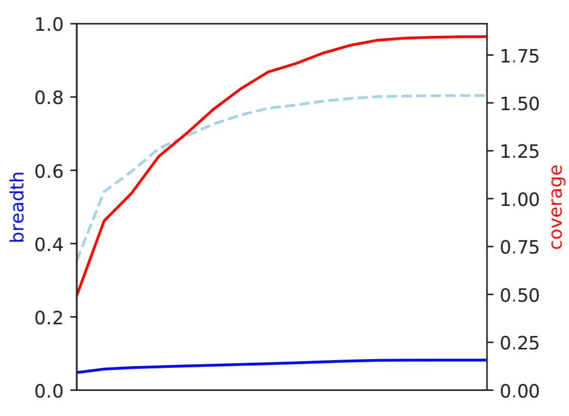
Breadth of coverage (blue line), coverage depth (red line), and expected breadth of coverage given the depth of coverage (dotted blue line) versus the minimum ANI of mapped reads. Coverage depth continues to increase while breadth of plateaus, suggesting that all regions of the reference genome are not present in the reads being mapped.

2) Genome-wide microdiversity metrics¶

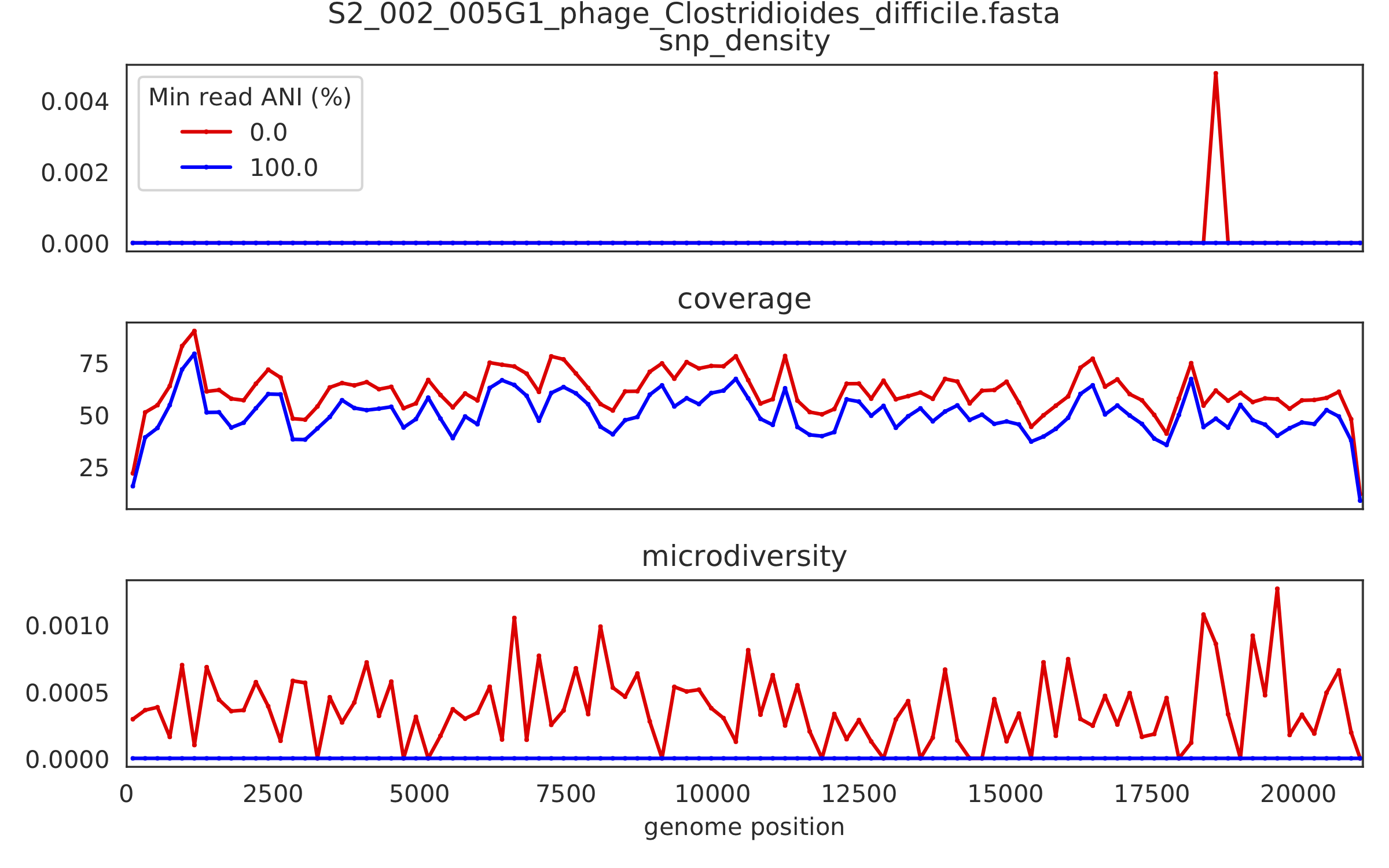
_images/genomeWide_microdiveristy_metrics_1.png

_images/genomeWide_microdiveristy_metrics_2.png

SNV density, coverage, and nucleotide diversity. Spikes in nucleotide diversity and SNV density do not correspond with increased coverage, indicating that the signals are not due to read mis-mapping. Positions with nucleotide diversity and no SNV-density are those where diversity exists but is not high enough to call a SNV

3) Read-level ANI distribution¶

Distribution of read pair ANI levels when mapped to a reference genome; this plot suggests that the reference genome is >1% different than the mapped reads

4) Major allele frequencies¶

Distribution of the major allele frequencies of bi-allelic SNVs (the Site Frequency Spectrum). Alleles with major frequencies below 50% are the result of multiallelic sites. The lack of distinct puncta suggest that more than a few distinct strains are present.

5) Linkage decay¶

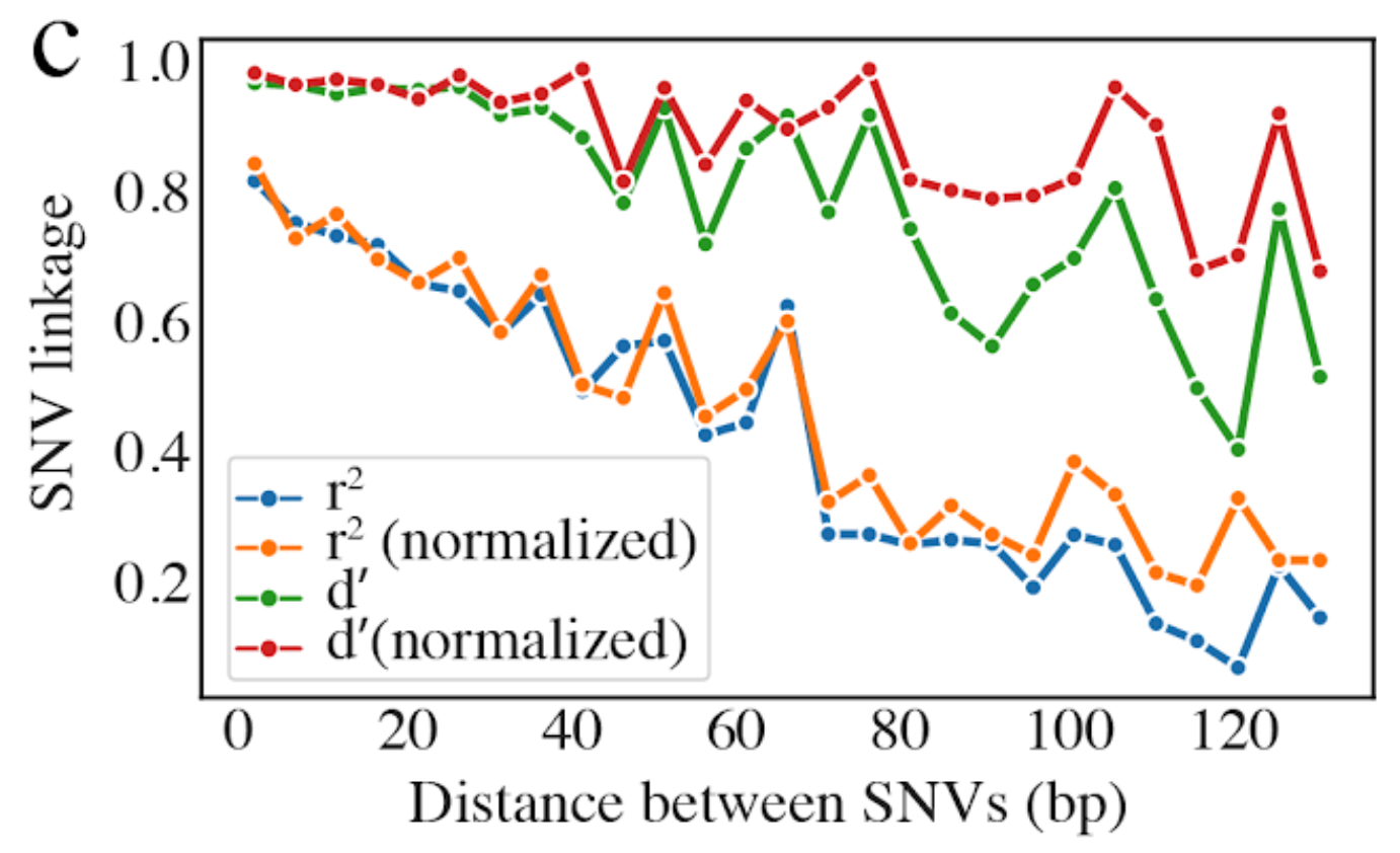
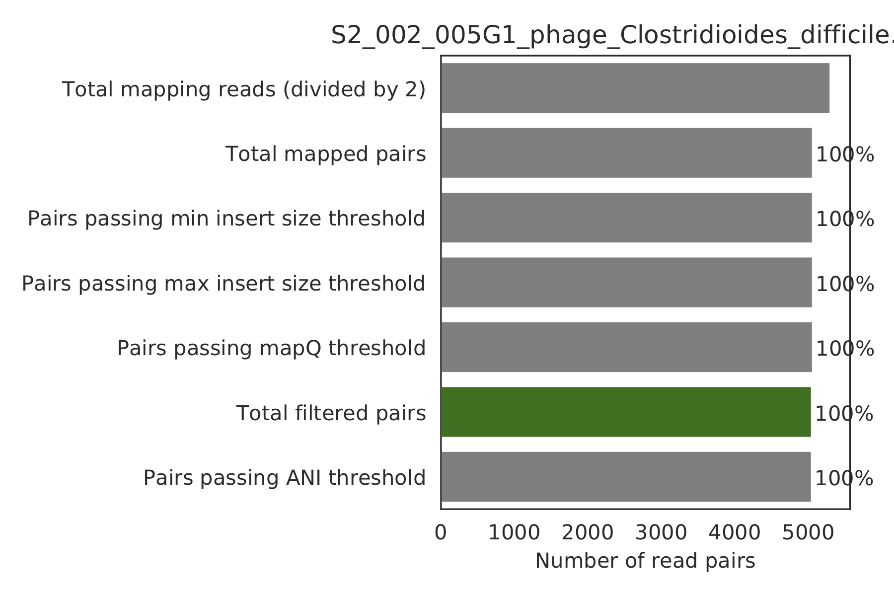
Metrics of SNV linkage vs. distance between SNVs; linkage decay (shown in one plot and not the other) is a common signal of recombination.

6) Read filtering plots¶

Bar plots showing how many reads got filtered out during filtering. All percentages are based on the number of paired reads; for an idea of how many reads were filtered out for being non-paired, compare the top bar and the second to top bar.

7) Scaffold inspection plot (large)¶

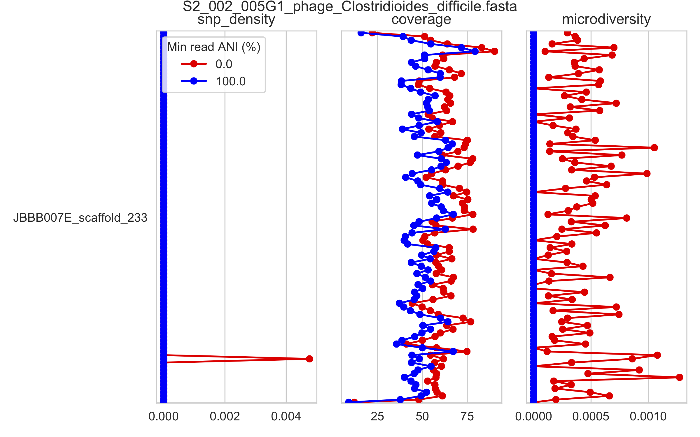
This is an elongated version of the genome-wide microdiversity metrics that is long enough for you to read scaffold names on the y-axis

8) Linkage with SNP type (GENES REQUIRED)¶

Linkage plot for pairs of non-synonymous SNPs and all pairs of SNPs

9) Gene histograms (GENES REQUIRED)¶

Histogram of values for all genes profiled

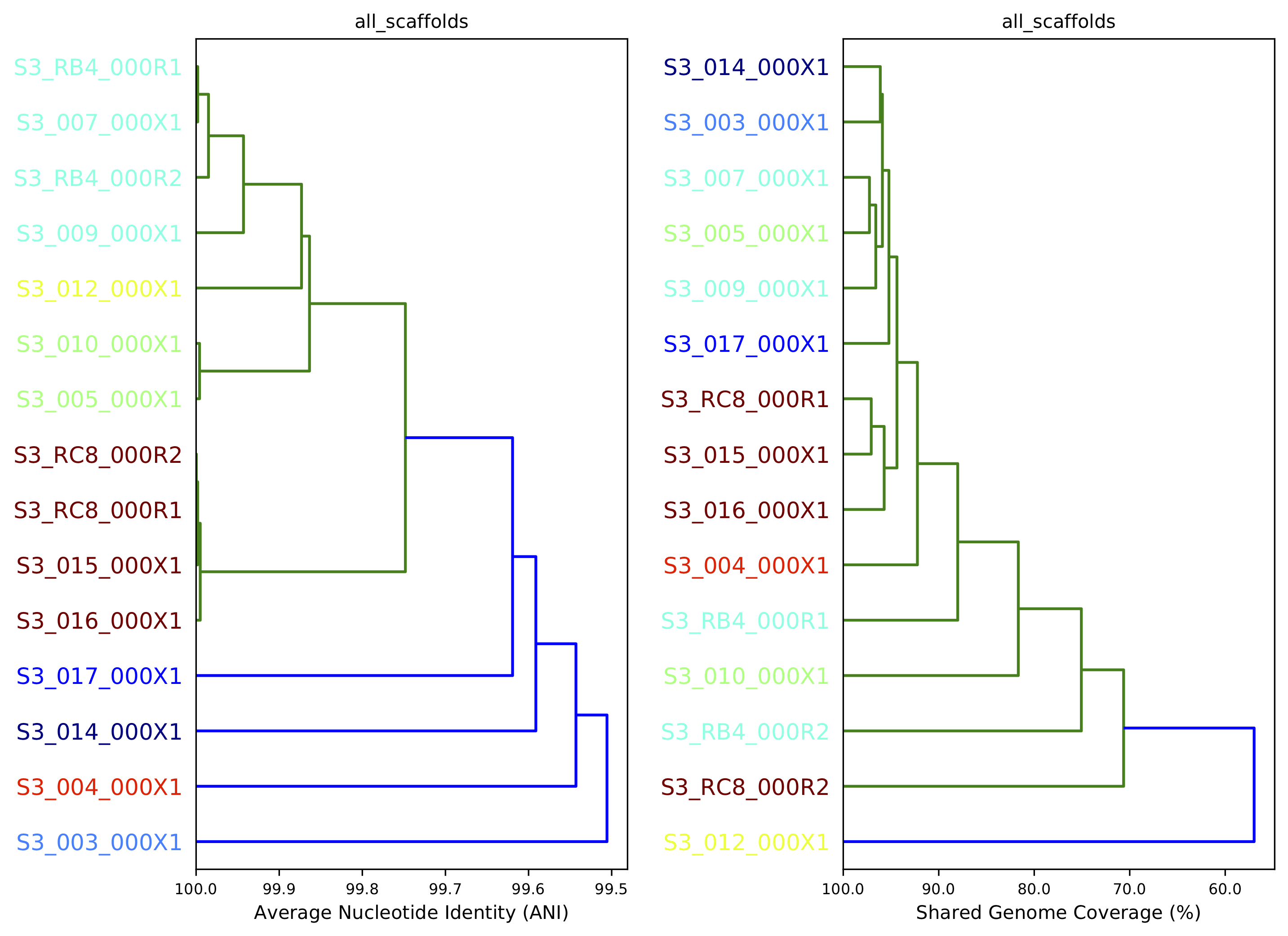
10) Compare dendrograms (RUN ON COMPARE; NOT PROFILE)¶

A dendrogram comparing all samples based on popANI and based on shared_bases.