Tutorial
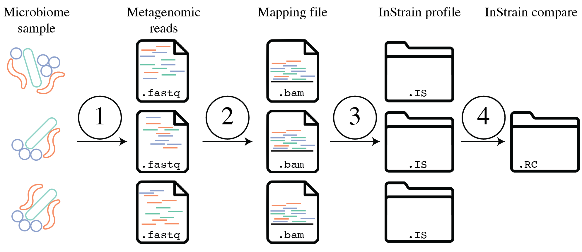
The above figure provides a conceptual overview of the steps involved when running inStrain. Step 1 is generating sequencing reads, step 2 is mapping those sequencing reads to a Genome database, step 3 is profiling the mapping with inStrain profile, step 4 is comparing inStrian profiles using inStrain compare.
Quick Start
The two main operations of inStrain are compare and profile.
Profile
InStrain profile takes as input a fasta file and a bam file and runs a series of steps to characterize the nucleotide diversity, SNSs and SNVs, linkage, etc.. If one provides a scaffold-to-bin file it will calculate genome-level metrics, and if one provides a genes file it will calculate gene level metrics.
The most basic inStrain profile command has this form:
$ inStrain profile .bam_file .fasta_file -o IS_output_name
Compare
InStrain compare takes as input multiple inStrain profile objects (generated using the command above) and performs strain-level comparisons. Each inStrain profile object used by InStrain compare must be made from reads mapped to the same fasta file.
The most basic inStrain compare command looks like this:
$ inStrain compare -i IS_output_1 IS_output_2 IS_output_3
Other
There are a number of other operations that inStrain can perform as well, although these generally perform more niche tasks. Check the program help (inStrain -h) to see a full list of the available operations
$ inStrain -h

                ...::: inStrain v1.4.0 :::...

  Matt Olm and Alex Crits-Christoph. MIT License. Banfield Lab, UC Berkeley. 2019

  Choose one of the operations below for more detailed help. See https://instrain.readthedocs.io for documentation.
  Example: inStrain profile -h

  Workflows:
    profile         -> Create an inStrain profile (microdiversity analysis) from a mapping.
    compare         -> Compare multiple inStrain profiles (popANI, coverage_overlap, etc.)

  Single operations:
    profile_genes   -> Calculate gene-level metrics on an inStrain profile [DEPRECATED; PROVIDE GENES TO profile]
    genome_wide     -> Calculate genome-level metrics on an inStrain profile [DEPRECATED; PROVIDE .stb FILES TO profile / compare]
    quick_profile   -> Quickly calculate coverage and breadth of a mapping using coverM
    filter_reads    -> Commands related to filtering reads from .bam files
    plot            -> Make figures from the results of "profile" or "compare"
    other           -> Other miscellaneous operations
See also
- Installation
To get started using the program
- User Manual
For descriptions of what the modules can do and information on how to prepare data for inStrain
- Expected output
To view example output and how to interpret it
Example inStrain commands
Running inStrain profile on a single genome
inStrain profile mappingfile.bam genomefile.fasta -o outputlocation.IS -p 6 -g genesfile.fasta
Running inStrain profile on a large set of genomes
inStrain profile mappingfile.bam genomesfile.fasta -o outputlocation.IS -p 6 -g genesfile.fasta -s scaffoldtobin.stb --database_mode
Running inStrain compare on a large set of genomes
inStrain compare -i genomefile-vs-sample1.IS/ genomefile-vs-sample2.IS/ -o genomefile.IS.COMPARE -p 6 -s scaffoldtobin.stb --database_mode
Tutorials
The following tutorials give step-by-step instructions on how to run inStrain a couple of different ways. The main difference between these tutorials is in how the Genome database used for inStrain analysis is generated. The user to inStrain decides on their own what genomes should be used for analysis, and there are a couple of broad options as depicted in the figure below.

Tutorial #1 uses test data that comes packaged with the inStrain source code to go through the basic steps of the program. It also describes how you can run using genomes that you have generated on your own.
Tutorial #2 describes how to run inStrain using an existing, public genome database. This way of running inStrain avoids the need for metagenomic assembly and genome binning.
Tutorial #3 describes how to combine custom genomes with an existing genome database. This allows users to include both sample-specific representative genomes and an existing genome database, and allows for comprehensive, accurate analysis.
Tutorial #1) Running inStrain on provided test data
The following tutorial goes through an example run of inStrain. You can follow along with your own data, or use a small set of reads that are included in the inStrain source code for testing. They can be found in the folder test/test_data/ of your install folder, or can be downloaded from the inStrain source code at this link on GitHub. The files that we’ll use for this tutorial are the forward and reverse metagenomic reads (N5_271_010G1.R1.fastq.gz and N5_271_010G1.R2.fastq.gz) and a .fasta file to map to (N5_271_010G1_scaffold_min1000.fa). In case you’re curious, these metagenomic reads come from a premature infant fecal sample.
Preparing input files
After downloading the genome file that you would like to profile (the fasta file) and at least one set of paired reads, the first thing to do is to map the reads to the .fasta file in order to generate a bam file.
When this mapping is performed it is important that you map to all genomes simultaneously (see Important concepts for why this is important). This involves combining all of the genomes that you’d like to map into a single .fasta file. In our case our .fasta file already has all of the genomes that we’d like to profile within it, but if you did want to profile a number of different genomes, you could combine them using a command like this
$ cat raw_data/S2_002_005G1_phage_Clostridioides_difficile.fasta raw_data/S2_018_020G1_bacteria_Clostridioides_difficile.fasta > allGenomes_v1.fasta
When we do this we also need to generate a file to let inStrain know which scaffolds came from which genomes. We can do this by giving inStrain a list of the .fasta files that went into making the concatenated .fasta file, or we can make a scaffold-to-bin file file, which lists the genome assignment of each scaffold in a tab-delimited file. This is how to do the later method using the parse_stb.py script that comes with the program dRep (Installed with the command pip install drep --upgrade)
$ parse_stb.py --reverse -f raw_data/S2_002_005G1_phage_Clostridioides_difficile.fasta raw_data/S2_018_020G1_bacteria_Clostridioides_difficile.fasta -o genomes.stb
Next we must map our reads to this fasta file to create bam files. In this tutorial we will use the mapping program Bowtie 2
$ mkdir bt2

$ bowtie2-build ~/Programs/inStrain/test/test_data/N5_271_010G1_scaffold_min1000.fa bt2/N5_271_010G1_scaffold_min1000.fa

$ bowtie2 -p 6 -x bt2/N5_271_010G1_scaffold_min1000.fa -1 ~/Programs/inStrain/test/test_data/N5_271_010G1.R1.fastq.gz -2 ~/Programs/inStrain/test/test_data/N5_271_010G1.R2.fastq.gz > N5_271_010G1_scaffold_min1000.fa-vs-N5_271_010G1.sam
At this point we have generated a .sam file, the precursor to .bam files. Lets make sure it’s there and not empty
$ ls -lht

total 34944
-rw-r--r--  1 mattolm  staff    16M Jan 23 11:56 N5_271_010G1_scaffold_min1000.fa-vs-N5_271_010G1.sam
drwxr-xr-x  8 mattolm  staff   256B Jan 23 11:54 bt2/
Perfect. At this point we could convert the .sam file to a sorted and indexed .bam file using samtools, but since inStrain can do that for us automatically we won’t bother.
If we want inStrain to do gene-level profiling we need to give it a list of genes to profile. Note - this is an optional step that is not required for inStrain to work in general, but without this you will not get gene-level profiles
We will profile our genes using the program prodigal, which can be run using the following example command
$ prodigal -i ~/Programs/inStrain/test/test_data/N5_271_010G1_scaffold_min1000.fa -d N5_271_010G1_scaffold_min1000.fa.genes.fna -a N5_271_010G1_scaffold_min1000.fa.genes.faa
Running inStrain profile
Now that we’ve gotten everything set up it’s time to run inStrain. To see all of the options, run
$ inStrain profile -h
A long list of arguments and options will show up. For more details on what these do, see User Manual. The only arguments that are absolutely required, however, are a .sam or .bam mapping file, and the .fasta file that the mapping file is mapped to.
Note
In this case we’re going to have inStrain profile the mapping, call genes, make the results genome wide, and plot the results all in one command. This is the recommended way to do things for the most computational efficiency. The other, not recommended way would be to run these all as separate steps (using the subcommands inStrain profile, inStrain profile_genes, inStrain genome_wide, and inStrain plot). See User Manual for more information.
Using all of the files we generated above, here is going to be our inStrain command
$ inStrain profile N5_271_010G1_scaffold_min1000.fa-vs-N5_271_010G1.sam ~/Programs/inStrain/test/test_data/N5_271_010G1_scaffold_min1000.fa -o N5_271_010G1_scaffold_min1000.fa-vs-N5_271_010G1.IS -p 6 -g N5_271_010G1_scaffold_min1000.fa.genes.fna -s ~/Programs/inStrain/test/test_data/N5_271_010G1.maxbin2.stb
You should see the following as inStrain runs (should only take a few minutes)
You gave me a sam- I'm going to make it a .bam now
Converting N5_271_010G1_scaffold_min1000.fa-vs-N5_271_010G1.sam to N5_271_010G1_scaffold_min1000.fa-vs-N5_271_010G1.ba
m
samtools view -S -b N5_271_010G1_scaffold_min1000.fa-vs-N5_271_010G1.sam > N5_271_010G1_scaffold_min1000.fa-vs-N5_271_
010G1.bam
sorting N5_271_010G1_scaffold_min1000.fa-vs-N5_271_010G1.bam
samtools sort N5_271_010G1_scaffold_min1000.fa-vs-N5_271_010G1.bam -o N5_271_010G1_scaffold_min1000.fa-vs-N5_271_010G1
.sorted.bam -@ 6
[bam_sort_core] merging from 0 files and 6 in-memory blocks...
Indexing N5_271_010G1_scaffold_min1000.fa-vs-N5_271_010G1.sorted.bam
samtools index N5_271_010G1_scaffold_min1000.fa-vs-N5_271_010G1.sorted.bam N5_271_010G1_scaffold_min1000.fa-vs-N5_271_
010G1.sorted.bam.bai -@ 6
***************************************************
    ..:: inStrain profile Step 1. Filter reads ::..
***************************************************

Filtering reads: 100%|██████████████████████████████████████████████████████████████| 178/178 [00:02<00:00, 70.99it/s]
37.3% of reads were removed during filtering
1,727 read pairs remain (0.0004472 Gbp)
***************************************************
.:: inStrain profile Step 2. Profile scaffolds ::..
***************************************************

Profiling splits: 100%|█████████████████████████████████████████████████████████████████| 7/7 [00:05<00:00,  1.21it/s]
Merging splits and profiling genes: 100%|███████████████████████████████████████████████| 7/7 [00:08<00:00,  1.18s/it]
***************************************************
.:: inStrain profile Step 4. Make genome-wide ::..
***************************************************

Scaffold to bin was made using .stb file
85.66% of scaffolds have a genome
93.82% of scaffolds have a genome
99.30% of scaffolds have a genome
***************************************************
 .:: inStrain profile Step 5. Generate plots ::..
***************************************************
making plots 1, 2, 3, 4, 5, 6, 7, 8, 9
Plotting plot 1
Plotting plot 2
85.66% of scaffolds have a genome
Plotting plot 3
57.37% of scaffolds have a genome
Plotting plot 4
97.33% of scaffolds have a genome
Plotting plot 5
Plotting plot 6
Plotting plot 7
97.33% of scaffolds have a genome
Plotting plot 8
94.32% of scaffolds have a genome
Plotting plot 9
$$$$$$$$$$$$$$$$$$$$$$$$$$$$$$$$$$$$$$$$$$$$$$$$$$$$$$$$$$$$$$$$$$$$$$$$$$$$$$$$

..:: inStrain profile finished ::..

Output tables........ N5_271_010G1_scaffold_min1000.fa-vs-N5_271_010G1.IS/output/
Figures.............. N5_271_010G1_scaffold_min1000.fa-vs-N5_271_010G1.IS/figures/
Logging.............. N5_271_010G1_scaffold_min1000.fa-vs-N5_271_010G1.IS/log/

See documentation for output descriptions - https://instrain.readthedocs.io/en/latest/

$$$$$$$$$$$$$$$$$$$$$$$$$$$$$$$$$$$$$$$$$$$$$$$$$$$$$$$$$$$$$$$$$$$$$$$$$$$$$$$$
The last but of the output shows you where the plots and figures have been made. Here’s a list of the files that you should see
$ ls -lht N5_271_010G1_scaffold_min1000.fa-vs-N5_271_010G1.IS/output/
total 91K
-rw-rw-r-- 1 mattolm infantgi  35K Jan 15 10:10 N5_271_010G1_scaffold_min1000.fa-vs-N5_271_010G1.IS_SNVs.tsv
-rw-rw-r-- 1 mattolm infantgi 1.2K Jan 15 10:10 N5_271_010G1_scaffold_min1000.fa-vs-N5_271_010G1.IS_genome_info.tsv
-rw-rw-r-- 1 mattolm infantgi  23K Jan 15 10:10 N5_271_010G1_scaffold_min1000.fa-vs-N5_271_010G1.IS_mapping_info.tsv
-rw-rw-r-- 1 mattolm infantgi  92K Jan 15 10:10 N5_271_010G1_scaffold_min1000.fa-vs-N5_271_010G1.IS_gene_info.tsv
-rw-rw-r-- 1 mattolm infantgi  15K Jan 15 10:10 N5_271_010G1_scaffold_min1000.fa-vs-N5_271_010G1.IS_linkage.tsv
-rw-rw-r-- 1 mattolm infantgi  30K Jan 15 10:10 N5_271_010G1_scaffold_min1000.fa-vs-N5_271_010G1.IS_scaffold_info.tsv

$ ls -lht N5_271_010G1_scaffold_min1000.fa-vs-N5_271_010G1.IS/figures/
total 3.5M
-rw-rw-r-- 1 mattolm infantgi 386K Jan 15 10:10 N5_271_010G1_scaffold_min1000.fa-vs-N5_271_010G1.IS_GeneHistogram_plot.pdf
-rw-rw-r-- 1 mattolm infantgi 379K Jan 15 10:10 N5_271_010G1_scaffold_min1000.fa-vs-N5_271_010G1.IS_LinkageDecay_types_plot.pdf
-rw-rw-r-- 1 mattolm infantgi 404K Jan 15 10:10 N5_271_010G1_scaffold_min1000.fa-vs-N5_271_010G1.IS_ScaffoldInspection_plot.pdf
-rw-rw-r-- 1 mattolm infantgi 375K Jan 15 10:10 N5_271_010G1_scaffold_min1000.fa-vs-N5_271_010G1.IS_ReadFiltering_plot.pdf
-rw-rw-r-- 1 mattolm infantgi 378K Jan 15 10:10 N5_271_010G1_scaffold_min1000.fa-vs-N5_271_010G1.IS_LinkageDecay_plot.pdf
-rw-rw-r-- 1 mattolm infantgi 377K Jan 15 10:10 N5_271_010G1_scaffold_min1000.fa-vs-N5_271_010G1.IS_MajorAllele_frequency_plot.pdf
-rw-rw-r-- 1 mattolm infantgi 375K Jan 15 10:10 N5_271_010G1_scaffold_min1000.fa-vs-N5_271_010G1.IS_readANI_distribution.pdf
-rw-rw-r-- 1 mattolm infantgi 400K Jan 15 10:10 N5_271_010G1_scaffold_min1000.fa-vs-N5_271_010G1.IS_genomeWide_microdiveristy_metrics.pdf
-rw-rw-r-- 1 mattolm infantgi 376K Jan 15 10:10 N5_271_010G1_scaffold_min1000.fa-vs-N5_271_010G1.IS_CoverageAndBreadth_vs_readMismatch.pdf
We have now successfully generated an inStrain profile! For help interpreting the output files, see Expected output
Running inStrain parse_annotations
InStrain parse_annotations creates output files that make it easier to perform functional gene analysis. One input file is the InStrain profile object, which we just created above, and the other input file is a table of gene annotations.
You can annotate your genes using whatever gene annotation database you like (depending on your specific project and questions). The section Gene Annotation in User Manual has instructions for a few databases. In this tutorial let’s just annotate with KEGG Orthologies (KOs) and Carbohydrate-Active enZYmes (CAZymes).
To do the annotations we’ll need the amino acid sequences of the genes (the file ending in .faa, created using the prodigal command above) even though the gene nucleotide sequences is what we provided to inStrain profile. Following the section Gene Annotation in User Manual, we’ll then run the following commands
$ exec_annotation -p profiles -k ko_list --cpu 10 --tmp-dir ./tmp -o N5_271_010G1_scaffold_min1000.fa.genes.faa.KO N5_271_010G1_scaffold_min1000.fa.genes.faa

$ hmmscan --domtblout N5_271_010G1_scaffold_min1000.fa.genes.faa_vs_dbCAN_v11.dm dbCAN-HMMdb-V11.txt N5_271_010G1_scaffold_min1000.fa.genes.faa > /dev/null ; sh /hmmscan-parser.sh N5_271_010G1_scaffold_min1000.fa.genes.faa_vs_dbCAN_v11.dm > N5_271_010G1_scaffold_min1000.fa.genes.faa_vs_dbCAN_v11.dm.ps ; cat N5_271_010G1_scaffold_min1000.fa.genes.faa_vs_dbCAN_v11.dm.ps | awk '$5<1e-15&&$10>0.35' > N5_271_010G1_scaffold_min1000.fa.genes.faa_vs_dbCAN_v11.dm.ps.stringent
We’ll now need to use python / R / Excel to parse and re-format the output of these (and any other) annotations. In the end they need be transformed into a single .csv file with the columns “gene” and “anno”. See User Manual for more details on the specific formatting requirements. In our case the file, which I called geneAnnotations_v1.csv, should look like this:
gene |
anno |
N5_271_010G1_scaffold_12_3 |
K06956 |
N5_271_010G1_scaffold_14_1 |
K09890 |
N5_271_010G1_scaffold_15_2 |
K07482 |
N5_271_010G1_scaffold_19_7 |
K09890 |
N5_271_010G1_scaffold_25_1 |
K20386 |
N5_271_010G1_scaffold_25_1 |
K15558 |
N5_271_010G1_scaffold_25_1 |
K19762 |
N5_271_010G1_scaffold_25_2 |
K06864 |
N5_271_010G1_scaffold_28_3 |
K07482 |
Now we can run inStrain parse_annotations with a command like the following
$ inStrain parse_annotations -i N5_271_010G1_scaffold_min1000.fa-vs-N5_271_010G1.IS/ -o genes_output_v1 -a geneAnnotations_v1.csv
Done! To see what output files you can expect, see Expected output
Running inStrain compare
InStrain compare compares genomes that have been profiled by multiple different metagenomic mappings. To compare genomes in the sample we just profiled above, we need to generate another bam file of reads from another sample to the same .fasta file. Provided in the inStrain test_data folder is exactly that- another different set of reads mapped to the same .fasta file (N5_271_010G1_scaffold_min1000.fa-vs-N5_271_010G2.sorted.bam). Let’s run inStrain on this to make a new inStrain profile
$ inStrain profile test_data/N5_271_010G1_scaffold_min1000.fa-vs-N5_271_010G2.sorted.bam N5_271_010G1_scaffold_min1000.fa -o N5_271_010G1_scaffold_min1000.fa-vs-N5_271_010G2.IS -p 6 -g N5_271_010G1_scaffold_min1000.fa.genes.fna -s N5_271_010G1.maxbin2.stb
To see the help section for inStrain compare run:
$ inStrain compare -h
As above, this will print out a whole list of parameters that can be turned depending on your specific use-case. Important concepts and User Manual provide some insight into what these parameters do and how to tune them. For the purposes of this tutorial we’re going to use mostly default parameters, giving us the following command
$ inStrain compare -i N5_271_010G1_scaffold_min1000.fa-vs-N5_271_010G1.IS/ N5_271_010G1_scaffold_min1000.fa-vs-N5_271_010G2.IS/ -s .N5_271_010G1.maxbin2.stb -p 6 -o N5_271_010G1_scaffold_min1000.fa.IS.COMPARE
This command should produce the following output
Scaffold to bin was made using .stb file
***************************************************
    ..:: inStrain compare Step 1. Load data ::..
***************************************************

Loading Profiles into RAM: 100%|████████████████████████████████████████████████████████| 2/2 [00:00<00:00, 67.45it/s]
158 of 167 scaffolds are in at least 2 samples
***************************************************
..:: inStrain compare Step 2. Run comparisons ::..
***************************************************

Running group 1 of 1
Comparing scaffolds: 100%|██████████████████████████████████████████████████████████| 158/158 [00:04<00:00, 36.12it/s]
***************************************************
..:: inStrain compare Step 3. Auxiliary processing ::..
***************************************************

***************************************************
..:: inStrain compare Step 4. Store results ::..
***************************************************

making plots 10
Plotting plot 10
/home/mattolm/.pyenv/versions/3.6.10/lib/python3.6/site-packages/inStrain/plottingUtilities.py:963: UserWarning: FixedFormatter should only be used together with FixedLocator
  axes.set_xticklabels(labels)
/home/mattolm/.pyenv/versions/3.6.10/lib/python3.6/site-packages/inStrain/plottingUtilities.py:963: UserWarning: FixedFormatter should only be used together with FixedLocator
  axes.set_xticklabels(labels)
Done!
$$$$$$$$$$$$$$$$$$$$$$$$$$$$$$$$$$$$$$$$$$$$$$$$$$$$$$$$$$$$$$$$$$$$$$$$$$$$$$$$

..:: inStrain compare finished ::..

Output tables........ N5_271_010G1_scaffold_min1000.fa.IS.COMPARE/output/
Figures.............. N5_271_010G1_scaffold_min1000.fa.IS.COMPARE/figures/
Logging.............. N5_271_010G1_scaffold_min1000.fa.IS.COMPARE/log/

See documentation for output descriptions - https://instrain.readthedocs.io/en/latest/

$$$$$$$$$$$$$$$$$$$$$$$$$$$$$$$$$$$$$$$$$$$$$$$$$$$$$$$$$$$$$$$$$$$$$$$$$$$$$$$$
As before, the last part of the output shows you where the plots and figures have been made. Here’s a list of the files that you should see
$ ls -lht N5_271_010G1_scaffold_min1000.fa.IS.COMPARE/output/
total 14K
-rw-rw-r-- 1 mattolm infantgi 28K Jan 15 10:33 N5_271_010G1_scaffold_min1000.fa.IS.COMPARE_comparisonsTable.tsv
-rw-rw-r-- 1 mattolm infantgi 352 Jan 15 10:33 N5_271_010G1_scaffold_min1000.fa.IS.COMPARE_strain_clusters.tsv
-rw-rw-r-- 1 mattolm infantgi 554 Jan 15 10:33 N5_271_010G1_scaffold_min1000.fa.IS.COMPARE_genomeWide_compare.tsv

$ ls  -lht N5_271_010G1_scaffold_min1000.fa.IS.COMPARE/figures/
total 393K
-rw-rw-r-- 1 mattolm infantgi 376K Jan 15 10:33 N5_271_010G1_scaffold_min1000.fa.IS.COMPARE_inStrainCompare_dendrograms.pdf
Success! As before, for help interpreting this output see Expected output .
Tutorial #2) Running inStrain using a public genome database
If you don’t want to assemble and bin your metagenomic samples it is also possible to run inStrain using publicly available reference genomes. Here we will go through a tutorial on how to do this with the UHGG genome collection, a collection of all microbial species known to exist in the human gut. The steps in this tutorial could be repeated with any set of genomes though, including genomes assembled from non-industrialized human populations, as available at the following link - https://doi.org/10.5281/zenodo.7782709
Preparing a genome database
Note
The genome database created in this section is available for direct download at the following link - https://doi.org/10.5281/zenodo.4441269 . You can download those files directly and skip this section if you would like. This genome set is based on UHGG version 1 and was created on Jan 14, 2021.
Note
An alternative genome database that includes UHGG genomes AND genomes assembled from non-industrialized human populations is available for direct download at the following link - https://doi.org/10.5281/zenodo.7782709 . This genome set is described in the following publication - https://doi.org/10.1101/2022.03.30.486478
In order to create a genome database we need to download the genomes, create a scaffold-to-bin file, create a genes file, and merge all genomes into a single fasta file that we can make a bowtie2 mapping index out of. All genomes in a genome need to database need to be distinct from one another, but not too distinct. See section “Establishing and evaluating genome databases” in Important concepts for more info.
First we must download the UHGG genomes themselves. The FTP site is here, and metadata on genomes is genomes-all_metadata.tsv. Let’s download this metadata file using curl:
$ curl http://ftp.ebi.ac.uk/pub/databases/metagenomics/mgnify_genomes/human-gut/v1.0/genomes-all_metadata.tsv -o genomes-all_metadata.tsv
Now that we have this metadata file we need to download all species representative genomes. There are a number of ways to do this, but we’re going to do it by parsing the metadata table in unix. Running the following command will 1) identify columns of species representatives, 2) parse the row to determine their FTP location, 3) create and run a curl command to download the genome:
$ cat genomes-all_metadata.tsv | awk -F "\t" '{if ($17 == $1) print "curl ftp://ftp.ebi.ac.uk/pub/databases/metagenomics/mgnify_genomes/human-gut/v1.0/uhgg_catalogue/" substr($18,0,13) "/" $18 "/genome/" $18 ".fna -o UHGG_reps/" $1 ".fna"}' | bash
The following command will let us check and make sure that we downloaded all 4644 genomes:
$ ls UHGG_reps/ | wc -l
  4644
Next we need to create a scaffold-to-bin file. This can easily be done using the script parse_stb.py that comes with the program dRep:
$ parse_stb.py --reverse -f UHGG_reps/* -o UHGG.stb
Next we’ll profile the genes for each genome using Prodigal to create a genes file. This can be done on the concatenated genome file (created below) or on the individual genomes (as shown in this code chunk). The benefit of the later is that it allows Prodigal to be run in single genome mode, as opposed to metagenome mode, which can be more accurate:
$ mkdir UHGG_genes

$ cd UHGG_reps/

$ for genome in $(ls *.fna); do echo prodigal -i $genome -o ../UHGG_genes/$genome.genes -a ../UHGG_genes/$genome.gene.faa -d ../UHGG_genes/$genome.gene.fna -m -p single; done | parallel -j 6

$ cat UHGG_genes/*.gene.fna > UHGG_reps.genes.fna

$ cat UHGG_genes/*.gene.faa > UHGG_reps.genes.faa
Finally we need to concatenate all genomes together into a single fasta file and create a bowtie2 mapping index from it:
$ cat UHGG_reps/* > UHGG_reps.fasta

$ bowtie2-build UHGG_reps.fasta UHGG_reps.fasta.bt2 --large-index --threads 20
Mapping to the Genome Database
Here we will use the program Bowtie2 to align our reads to the reference database. If you downloaded the pre-made version of bowtie2 index, you’ll need to extract it using the following command
$ tar -zxvf UHGG_reps_v1.bt2.tgz
This should yield a set of 5 files that end in .bt2l
Next we need to map our metagenomic reads to the database. For the purposes of this tutorial we’ll use metagenomic reads that came from a premature infant fecal sample. The bowtie2 command to map these reads is
$ bowtie2 -p 10 -x /groups/banfield/projects/human/data8/ExternalData/UHGG/UHGG_reps.fasta.bt2 -1 /groups/banfield/projects/human/data8/raw.d/NIH5/reads/HR/N5_216_039G1_T0140F_S50_L002.HR.R1.fastq.gz -2 /groups/banfield/projects/human/data8/raw.d/NIH5/reads/HR/N5_216_039G1_T0140F_S50_L002.HR.R2.fastq.gz > UHGG_reps.fasta-vs-N5_216_039G1.sam

  7032881 reads; of these:
    7032881 (100.00%) were paired; of these:
      1690938 (24.04%) aligned concordantly 0 times
      1905098 (27.09%) aligned concordantly exactly 1 time
      3436845 (48.87%) aligned concordantly >1 times
      ----
      1690938 pairs aligned concordantly 0 times; of these:
        139804 (8.27%) aligned discordantly 1 time
      ----
      1551134 pairs aligned 0 times concordantly or discordantly; of these:
        3102268 mates make up the pairs; of these:
          1851642 (59.69%) aligned 0 times
          279669 (9.01%) aligned exactly 1 time
          970957 (31.30%) aligned >1 times
  86.84% overall alignment rate
This mapping took just over 10 minutes on my computer. Notice how the bowtie2 states that over 85% of reads align to the database- this is an important number to consider, as all reads that do not align to the database will be invisible to inStrain. For human microbiome samples 85% is pretty good, but performing de novo genome assembly and including sample-specific genomes would undoubtedly raise this number.
Running inStrain profile
Next we’ll profile the .sam file created above with inStrain. To do this we’ll need the scaffold-to-bin file, genes file, and fasta file for the database that we created in the first step. If you downloaded them you can decompress them with the commands
$ gzip -d UHGG_reps.fasta.gz

$ gzip -d UHGG_reps.genes.fna.gz
**When running inStrain on a big database like we have here it’s critical to add the flag --database mode. This flag does some quick calculations to figure out which genomes are probably not present, and stops working on them right away. This leads to dramatic reductions in RAM usage and computational time.
The inStrain profile command we’ll use now is
$ inStrain profile UHGG_reps.fasta-vs-N5_216_039G1.sam /groups/banfield/projects/human/data8/ExternalData/UHGG/UHGG_reps.fasta -o UHGG_reps.fasta-vs-N5_216_039G1.IS -p 10 -g /groups/banfield/projects/human/data8/ExternalData/UHGG/UHGG_reps.genes.fna -s /groups/banfield/projects/human/data8/ExternalData/UHGG/UHGG_reps.stb --database_mode
This took just over an hour to run on my computer. We have now successfully generated an inStrain profile! For help interpreting the output files, see Expected output. To link the genomes in the UHGG database with their taxonomy, use the file genomes-nr_metadata.tsv which we downloaded above and is part of the overall download as well. To subset to just the species representative genomes (SRGs) that make up this database, subset this table to only include rows where the column “Genome” is equal to the column “Species_rep”.
Running inStrain compare
InStrain compare compare genomes that have been profiled by multiple different metagenomic mappings. To compare genomes in the sample we just profiled above, we need to generate another bam file of reads from another sample to the same .fasta file. For example, something like the command (based on reads from this fecal sample from the same premature infant):
bowtie2 -p 10 -x /groups/banfield/projects/human/data8/ExternalData/UHGG/UHGG_reps.fasta.bt2 -1 /groups/banfield/projects/human/data8/raw.d/NIH5/reads/HR/N5_216_046G1_T0140F_S50_L002.HR.R1.fastq.gz -2 /groups/banfield/projects/human/data8/raw.d/NIH5/reads/HR/N5_216_046G1_T0140F_S50_L002.HR.R2.fastq.gz > UHGG_reps.fasta-vs-N5_216_046G1.sam

$ inStrain profile UHGG_reps.fasta-vs-N5_216_046G1.sam /groups/banfield/projects/human/data8/ExternalData/UHGG/UHGG_reps.fasta -o UHGG_reps.fasta-vs-N5_216_046G1.IS -p 10 -g /groups/banfield/projects/human/data8/ExternalData/UHGG/UHGG_reps.genes.fna -s /groups/banfield/projects/human/data8/ExternalData/UHGG/UHGG_reps.stb --database_mode
Now that we have two inStrain profile objects based on reads mapped to the same .fasta file, we can compare all detected genomes using the following command:
inStrain compare -i UHGG_reps.fasta-vs-N5_216_039G1.IS/ UHGG_reps.fasta-vs-N5_216_046G1.IS/ -s /groups/banfield/projects/human/data8/ExternalData/UHGG/UHGG_reps.stb -p 6 -o UHGG_reps.fasta.IS.COMPARE --database_mode
Success! As before, for help interpreting this output see Expected output.
Tutorial #3) Merging custom genomes with an existing genome database.
Using a combination of sample-specific genomes for accuracy and public genome databases for comprehensiveness can provide the best of both worlds. The steps are as follows:
Establish a set of data-set specific genomes through de novo genome assembly and binning. This could be done using a tool such as anvi’o, for example.
Download an entire database of individual genomes. See the top of Tutorial #2 for instructions on downloading UHGG.
Dereplicate both sets of genomes. The specific threshold you use for dereplication is important and some thoughts about choosing thresholds is available at Important concepts. A program that can be used for this purpose is dRep; just make sure you have dRep version 3 which is able to handle much larger genome sets than previous versions. An example command that could be used for this step is
dRep dereplicate MergedGenomeSet -g FullListOfGenomes.txt –S_algorithm fastANI –multiround_primary_clustering –clusterAlg greedy -ms 10000 -pa 0.9 -sa 0.95 -nc 0.30 -cm larger -p 16
This command will result in a species-level dereplicated set of genomes that include both your custom genomes and the database genomes. More details on genome dereplication can be found here. To prioritize your custom genomes over the database genomes, use the flag extra_weight_table within dRep.
Create a genome database out of the genomes in the dereplicated_genomes folder produced in the step above. This can be done following the instructions at the top of Tutorial #2.