Example output and explanations

InStrain produces a variety of output in the IS folder depending on which operations are run. Generally, output that is meant for human eyes to be easily interpretable is located in the output folder.

inStrain profile

A typical run of inStrain will yield the following files in the output folder:

scaffold_info.tsv

This gives basic information about the scaffolds in your sample at the highest allowed level of read identity.

scaffold_info.tsv

scaffold	length	breadth	coverage	coverage_median	coverage_std	bases_w_0_coverage	mean_clonality	median_clonality	mean_microdiversity	median_microdiversity	unmaskedBreadth	breadth_expected	SNPs	Referece_SNPs	BiAllelic_SNPs	MultiAllelic_SNPs	consensus_SNPs	population_SNPs	conANI	popANI
S3_003_000X1_scaffold_21039	1049	0.9609151572926596	7.778836987607247	9	3.6242339424115295	41	0.9984115827692688	1.0	0.0015884172307313313	0.0	0.7836034318398475	0.9989601856174312	1	0	1	0	0	0	1.0	1.0
S3_003_000X1_scaffold_21063	1048	0.3721374045801527	0.6698473282442748	0	0.978669048484894	658					0.0	0.4464898509344126	0	0	0	0	0	0	0.0	0.0
S3_003_000X1_scaffold_21081	1047	0.2082139446036294	0.2082139446036294	0	0.4060306612513717	829					0.0	0.1679418203027453	0	0	0	0	0	0	0.0	0.0
S3_003_000X1_scaffold_21188	1043	0.3547459252157239	0.4688398849472674	0	0.6908089219842111	673					0.0	0.338989542420026	0	0	0	0	0	0	0.0	0.0
S3_003_000X1_scaffold_21225	1042	0.7821497120921305	4.341650671785029	5	3.4491608427332947	227	1.0	1.0	0.0	0.0	0.5374280230326296	0.9783700757950428	0	0	0	0	0	0	1.0	1.0

scaffold

The name of the scaffold in the input .fasta file

length

Full length of the scaffold in the input .fasta file

breadth

The percentage of bases in the scaffold that are covered by at least a single read. A breadth of 1 means that all bases in the scaffold have at least one read covering them

coverage

The average depth of coverage on the scaffold. If half the bases in a scaffold have 5 reads on them, and the other half have 10 reads, the coverage of the scaffold will be 7.5

coverage_median

The median coverage value of all bases in the scaffold, included bases with 0 coverage

coverage_std

The standard deviation of all coverage values

bases_w_0_coverage

The number of bases with 0 coverage

mean_clonality

The mean clonality value of all bases in the scaffold that have a clonality value calculated. So if only 1 base on the scaffold meats the minimum coverage to calculate clonality, the mean_clonality of the scaffold will be the clonality of that base

median_clonality

The median clonality value of all bases in the scaffold that have a clonality value calculated

mean_microdiversity

The mean mean_microdiversity value of all bases in the scaffold that have a mean_microdiversity value calculated (microdiveristy = 1 - clonality)

median_microdiversity

The median microdiversity value of all bases in the scaffold that have a microdiversity value calculated

unmaskedBreadth

The percentage of bases in the scaffold that have at least the min_cov number of bases. This value multiplied by the length of the scaffold gives the percentage of bases for which clonality is calculated and on which SNPs can be called

SNPs

The total number of SNPs called on this scaffold

breadth_expected

This tells you the breadth that you should expect if reads are evenly distributed along the genome, given the reported coverage value. Based on the function breadth = -1.000 * e^(0.883 * coverage) + 1.000. This is useful to establish whether or not the scaffold is actually in the reads, or just a fraction of the scaffold. If your coverage is 10x, the expected breadth will be ~1. If your actual breadth is significantly lower then the expected breadth, this means that reads are mapping only to a specific region of your scaffold (transposon, etc.)

SNPs

The total number of SNPs called on this scaffold

Referece_SNPs

The number of SNPs called on this scaffold with allele_count = 1. This means that the only allele detected in the reads is different from the reference base

BiAllelic_SNPs

The number of SNPs called on this scaffold with allele_count = 2. This means that there are two possible alleles at this position

MultiAllelic_SNPs

The number of SNPs called on this scaffold with allele_count > 2. This means that there are more than two possible alleles at this position

consensus_SNPs

The number of SNPs called on this scaffold with allele_count > 0 and where consensus base is not the reference base. This should be the same as Reference_SNPs under almost all circumstances

population_SNPs

These are SNPs where the reference base isn’t detected at all, regardless of the allele count.

conANI

The average nucleotide identity between the reads in the sample and the .fasta file based on consensus SNPs. Calculated using the formula ANI = (unmaskedBreadth * length) - consensus_SNPs)/ (unmaskedBreadth * length))

popANI

The average nucleotide identity between the reads in the sample and the .fasta file based on consensus SNPs. Calculated using the formula ANI = (unmaskedBreadth * length) - population_SNPs)/ (unmaskedBreadth * length))

mapping_info.tsv

This provides an overview of the number of reads that map to each scaffold, and some basic metrics about their quality.

mapping_info.tsv

scaffold	unfiltered_reads	unfiltered_pairs	pass_filter_cutoff	pass_max_insert	pass_min_insert	pass_min_mapq	filtered_pairs	mean_mistmaches	mean_insert_distance	mean_mapq_score	mean_pair_length	median_insert	mean_PID
all_scaffolds	3802370	1790817	1674511	1784011	1790699	1790817	1668496	2.7480758782164787	293.0713925543481	23.46918082640493	298.38404705785126	246.0	0.9906729188638016
S3_002_000X1_scaffold_1162	12	6	6	6	6	6	6	1.0	281.1666666666667	25.16666666666667	300.0	287.0	0.9966666666666668
S3_002_000X1_scaffold_1005	10	5	5	5	5	5	5	0.2	318.0	33.2	299.8	208.0	0.9993333333333332
S3_002_000X1_scaffold_1151	6	3	3	3	3	3	3	5.666666666666668	280.3333333333333	19.666666666666668	300.0	293.0	0.9811111111111112
S3_002_000X1_scaffold_1004	14	6	6	6	6	6	6	0.5	295.5	16.666666666666668	300.0	248.0	0.9983333333333334

The following metrics are provided for all individual scaffolds, and for all scaffolds together (scaffold “all_scaffolds”). For the max insert cutoff, the median_insert for all_scaffolds is used

header line

The header line (starting with #; not shown in the above table) describes the parameters that were used to filter the reads

scaffold

The name of the scaffold in the input .fasta file

unfiltered_reads

The raw number of reads that map to this scaffold

unfiltered_pairs

The raw number of pairs of reads that map to this scaffold. Only paired reads are used by inStrain

pass_filter_cutoff

The number of pairs of reads mapping to this scaffold that pass the ANI filter cutoff (specified in the header as “filter_cutoff”)

pass_max_insert

The number of pairs of reads mapping to this scaffold that pass the maximum insert size cutoff- that is, their insert size is less than 3x the median insert size of all_scaffolds. Note that the insert size is measured from the start of the first read to the end of the second read (2 perfectly overlapping 50bp reads will have an insert size of 50bp)

pass_min_insert

The number of pairs of reads mapping to this scaffold that pass the minimum insert size cutoff

pass_min_mapq

The number of pairs of reads mapping to this scaffold that pass the minimum mapQ score cutoff

filtered_pairs

The number of pairs of reads that pass all cutoffs

mean_mistmaches

Among all pairs of reads mapping to this scaffold, the mean number of mismatches

mean_insert_distance

Among all pairs of reads mapping to this scaffold, the mean insert distance. Note that the insert size is measured from the start of the first read to the end of the second read (2 perfectly overlapping 50bp reads will have an insert size of 50bp)

mean_mapq_score

Among all pairs of reads mapping to this scaffold, the average mapQ score

mean_pair_length

Among all pairs of reads mapping to this scaffold, the average length of both reads in the pair summed together

median_insert

Among all pairs of reads mapping to this scaffold, the median insert distance.

mean_PID

Among all pairs of reads mapping to this scaffold, the average percentage ID of both reads in the pair to the reference .fasta file

SNVs.tsv

This describes the SNPs that are detected in this mapping.

SNVs.tsv

scaffold	position	ref_base	A	C	T	G	con_base	var_base	allele_count	cryptic	position_coverage	var_freq	ref_freq
S3_003_000X1_scaffold_21039	833	C	2	7	0	0	C	A	2	False	9	0.2222222222222222	0.7777777777777778
S3_003_000X1_scaffold_20	99	C	0	0	5	0	T	A	1	False	5	0.0	1.0
S3_003_000X1_scaffold_20	123	A	0	0	0	11	G	A	1	False	11	0.0	1.0
S3_003_000X1_scaffold_20	261	T	19	0	0	0	A	A	1	False	19	1.0	1.0
S3_003_000X1_scaffold_20	291	C	0	16	2	0	C	T	2	False	18	0.1111111111111111	0.8888888888888888

See the module_descriptions for what constitutes a SNP (what makes it into this table)

scaffold

The scaffold that the SNP is on

position

The genomic position of the SNP

ref_base

The reference base in the .fasta file at that position

A, C, T, and G

The number of mapped reads encoding each of the bases

con_base

The consensus base; the base that is supported by the most reads

var_base

Variant base; the base with the second most reads

morphia

The number of bases that are detected above background levels. In order to be detected above background levels, you must pass an fdr filter. See module descriptions for a description of how that works. A morphia of 0 means no bases are supported by the reads, a morphia of 1 means that only 1 base is supported by the reads, a morphia of 2 means two bases are supported by the reads, etc.

cryptic

If a SNP is cryptic, it means that it is detected when using a lower read mismatch threshold, but becomes undetected when you move to a higher read mismatch level. See “dealing with mm” in the advanced_use section for more details on what this means.

position_coverage

The total number of reads at this position

var_freq

The fraction of reads supporting the var_base

ref_freq

The fraction of reds supporting the ref_base

con_freq

The fraction of reds supporting the con_base

linkage.tsv

This describes the linkage between pairs of SNPs in the mapping that are found on the same read pair at least min_snp times.

linkage.tsv

r2	d_prime	r2_normalized	d_prime_normalized	total	countAB	countAb	countaB	countab	allele_A	allele_a	allele_B	allele_b	distance	position_A	position_B	scaffold
1.0	1.0	1.0	1.0	27	0	14	13	0	G	A	T	C	45	191425	191470	S3_003_000X1_scaffold_20
0.10743801652892566	1.0000000000000002	0.05263157894736843	1.0	24	13	0	9	2	G	A	C	A	80	191425	191505	S3_003_000X1_scaffold_20
0.08333333333333348	1.0	0.07894736842105264	1.0	26	11	2	13	0	T	C	C	A	35	191470	191505	S3_003_000X1_scaffold_20
1.0000000000000009	1.0	1.0	1.0	30	22	0	0	8	C	T	T	C	12	99342	99354	S3_003_000X1_scaffold_88
1.0000000000000004	1.0	1.0	1.0	22	17	0	0	5	C	T	T	A	60	99342	99402	S3_003_000X1_scaffold_88

Linkage is used primarily to determine if organisms are undergoing horizontal gene transfer or not. It’s calculated for pairs of SNPs that can be connected by at least min_snp reads. It’s based on the assumption that each SNP as two alleles (for example, a A and b B). This all gets a bit confusing and has a large amount of literature around each of these terms, but I’ll do my best to briefly explain what’s going on

scaffold

The scaffold that both SNPs are on

position_A

The position of the first SNP on this scaffold

position_B

The position of the second SNP on this scaffold

distance

The distance between the two SNPs

allele_A

One of the two bases at position_A

allele_a

The other of the two bases at position_A

allele_B

One of the bases at position_B

allele_b

The other of the two bases at position_B

countAB

The number of read-pairs that have allele_A and allele_B

countAb

The number of read-pairs that have allele_A and allele_b

countaB

The number of read-pairs that have allele_a and allele_B

countab

The number of read-pairs that have allele_a and allele_b

total

The total number of read-pairs that have have information for both position_A and position_B

r2

This is the r-squared linkage metric. See below for how it’s calculated

d_prime

This is the d-prime linkage metric. See below for how it’s calculated

r2_normalized, d_prime_normalized

These are calculated by rarefying to min_snp number of read pairs. See below for how it’s calculated

Python code for the calculation of these metrics:

freq_AB = float(countAB) / total
freq_Ab = float(countAb) / total
freq_aB = float(countaB) / total
freq_ab = float(countab) / total

freq_A = freq_AB + freq_Ab
freq_a = freq_ab + freq_aB
freq_B = freq_AB + freq_aB
freq_b = freq_ab + freq_Ab

linkD = freq_AB - freq_A * freq_B

if freq_a == 0 or freq_A == 0 or freq_B == 0 or freq_b == 0:
    r2 = np.nan
else:
    r2 = linkD*linkD / (freq_A * freq_a * freq_B * freq_b)

linkd = freq_ab - freq_a * freq_b

# calc D-prime
d_prime = np.nan
if (linkd < 0):
    denom = max([(-freq_A*freq_B),(-freq_a*freq_b)])
    d_prime = linkd / denom

elif (linkD > 0):
    denom = min([(freq_A*freq_b), (freq_a*freq_B)])
    d_prime = linkd / denom

################
# calc rarefied

rareify = np.random.choice(['AB','Ab','aB','ab'], replace=True, p=[freq_AB,freq_Ab,freq_aB,freq_ab], size=min_snp)
freq_AB = float(collections.Counter(rareify)['AB']) / min_snp
freq_Ab = float(collections.Counter(rareify)['Ab']) / min_snp
freq_aB = float(collections.Counter(rareify)['aB']) / min_snp
freq_ab = float(collections.Counter(rareify)['ab']) / min_snp

freq_A = freq_AB + freq_Ab
freq_a = freq_ab + freq_aB
freq_B = freq_AB + freq_aB
freq_b = freq_ab + freq_Ab

linkd_norm = freq_ab - freq_a * freq_b

if freq_a == 0 or freq_A == 0 or freq_B == 0 or freq_b == 0:
    r2_normalized = np.nan
else:
    r2_normalized = linkd_norm*linkd_norm / (freq_A * freq_a * freq_B * freq_b)


# calc D-prime
d_prime_normalized = np.nan
if (linkd_norm < 0):
    denom = max([(-freq_A*freq_B),(-freq_a*freq_b)])
    d_prime_normalized = linkd_norm / denom

elif (linkd_norm > 0):
    denom = min([(freq_A*freq_b), (freq_a*freq_B)])
    d_prime_normalized = linkd_norm / denom

rt_dict = {}
for att in ['r2', 'd_prime', 'r2_normalized', 'd_prime_normalized', 'total', 'countAB', \
            'countAb', 'countaB', 'countab', 'allele_A', 'allele_a', \
            'allele_B', 'allele_b']:
    rt_dict[att] = eval(att)

inStrain compare

A typical run of inStrain will yield the following files in the output folder:

comparisonsTable.tsv

scaffold	name1	name2	coverage_overlap	compared_bases_count	percent_genome_compared	length	consensus_SNPs	population_SNPs	conANI	popANI
S3_016_000X1_scaffold_14208	Sloan3AllGenomeInventory.fasta-vs-S3_003_000X1.sorted.bam	Sloan3AllGenomeInventory.fasta-vs-S3_016_000X1.sorted.bam	0.9825304393859184	1856	0.9814912744579588	1891	7	0	0.996228448275862	1.0
S3_016_000X1_scaffold_9493	Sloan3AllGenomeInventory.fasta-vs-S3_003_000X1.sorted.bam	Sloan3AllGenomeInventory.fasta-vs-S3_016_000X1.sorted.bam	0.9778541428025964	2561	0.977107974055704	2621	2	0	0.9992190550566185	1.0
S3_016_000X1_scaffold_12686	Sloan3AllGenomeInventory.fasta-vs-S3_003_000X1.sorted.bam	Sloan3AllGenomeInventory.fasta-vs-S3_016_000X1.sorted.bam	0.9787336877718704	2025	0.9768451519536904	2073	7	0	0.9965432098765432	1.0
S3_016_000X1_scaffold_11829	Sloan3AllGenomeInventory.fasta-vs-S3_003_000X1.sorted.bam	Sloan3AllGenomeInventory.fasta-vs-S3_016_000X1.sorted.bam	0.9739130434782608	2128	0.9712460063897764	2191	14	0	0.9934210526315792	1.0
S3_016_000X1_scaffold_8891	Sloan3AllGenomeInventory.fasta-vs-S3_003_000X1.sorted.bam	Sloan3AllGenomeInventory.fasta-vs-S3_016_000X1.sorted.bam	0.9826212889210716	2714	0.9826212889210716	2762	5	0	0.9981577008106116	1.0

scaffold

The scaffold being compared

name1

The name of the first inStrain profile being compared

name2

The name of the second inStrain profile being compared

coverage_overlap

The percentage of bases that are either covered or not covered in both of the profiles (covered = the base is present at at least min_snp coverage). The formula is length(coveredInBoth) / length(coveredInEither). If both scaffolds have 0 coverage, this will be 0.

compared_bases_count

The number of considered bases; that is, the number of bases with at least min_snp coverage in both profiles. Formula is length([x for x in overlap if x == True]).

percent_genome_compared

The percentage of bases in the scaffolds that are covered by both. The formula is length([x for x in overlap if x == True])/length(overlap). When ANI is np.nan, this must be 0. If both scaffolds have 0 coverage, this will be 0.

length

The total length of the scaffold

consensus_SNPs

The number of locations along the genome where both samples have the base at >= 5x coverage, and the consensus allele in each sample is different

population_SNPs

The number of locations along the genome where both samples have the base at >= 5x coverage, and no alleles are shared between either sample. See inStrain manuscript for more details.

popANI

The average nucleotide identity among compared bases between the two scaffolds, based on population_SNPs. Calculated using the formula popANI = (compared_bases_count - population_SNPs) / compared_bases_count

conANI

The average nucleotide identity among compared bases between the two scaffolds, based on consensus_SNPs. Calculated using the formula conANI = (compared_bases_count - consensus_SNPs) / compared_bases_count

inStrain profile_genes

A typical run of inStrain profile_genes will yield the following additional files in the output folder:

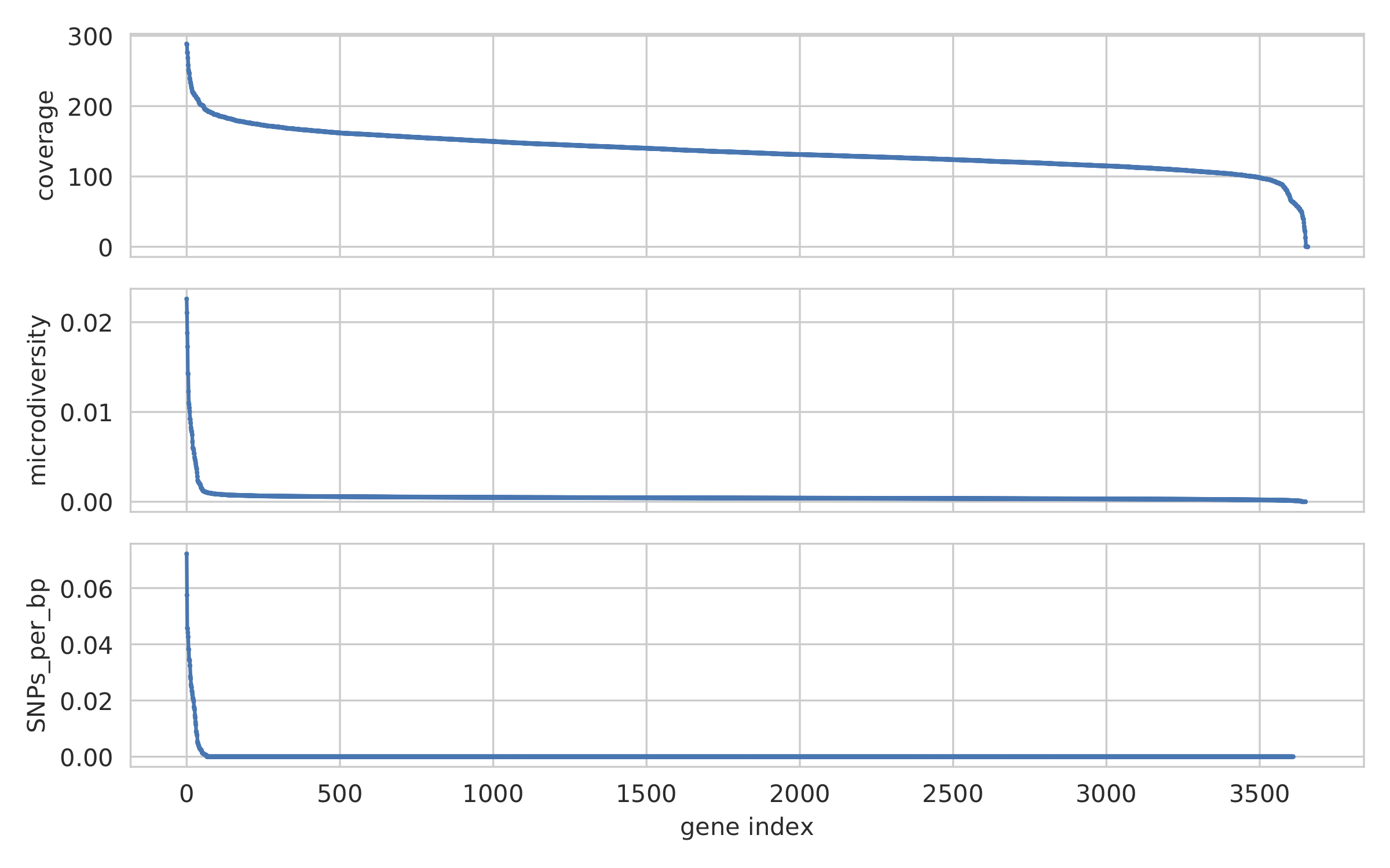
gene_info.tsv

This describes some basic information about the genes being profiled

gene_info.tsv

gene	scaffold	direction	partial	start	end	coverage	breadth	clonality	microdiversity	masked_breadth	SNPs_per_bp	min_ANI
S3_002_028G1_scaffold_0_1	S3_002_028G1_scaffold_0	-1	False	957	2219							0
S3_002_028G1_scaffold_0_2	S3_002_028G1_scaffold_0	-1	False	2189	3136							0
S3_002_028G1_scaffold_0_3	S3_002_028G1_scaffold_0	1	False	3274	5013							0
S3_002_028G1_scaffold_0_4	S3_002_028G1_scaffold_0	-1	False	5018	5746							0
S3_002_028G1_scaffold_0_5	S3_002_028G1_scaffold_0	1	False	5888	6862							0

gene

Name of the gene being profiled

scaffold

Scaffold that the gene is on

direction

Direction of the gene (based on prodigal call). If -1, means the gene is not coded in the direction expressed by the .fasta file

partial

If True this is a partial gene; based on not having partial=00 in the record description provided by Prodigal

start

Start of the gene (position on scaffold; 0-indexed)

end

End of the gene (position on scaffold; 0-indexed)

coverage

The mean coverage across the length of the gene

breadth

The number of bases in the gene that have at least 1x coverage

microdiversity

The mean nucleotide diversity (pi) among positions on the gene with at least 5x coverage

clonality

1 - microdiversity

masked_breadth

The percentage of positions in the gene with at least 5x coverage

SNPs_per_bp

The number of positions on the gene where a SNP is called

min_ANI

The minimum read ANI level when profile_genes was run (0 means the value is whatever was set with Profile was originally run)

SNP_mutation_types.tsv

This describes whether SNPs are synonymous, nonsynonymous, or intergenic

SNP_mutation_types.tsv

scaffold	position	ref_base	A	C	T	G	con_base	var_base	allele_count	position_coverage	var_freq	ref_freq	mutation_type	mutation	gene
S3_002_056W1_scaffold_121	2134	C	0	3	2	0	C	T	2	5	0.4	0.6	N	N:H936Y	S3_002_056W1_scaffold_121_2
S3_002_056W1_scaffold_121	8509	G	7	0	0	0	A	A	1	7	1.0	1.0	N	N:G459R	S3_002_056W1_scaffold_121_11
S3_002_056W1_scaffold_121	8510	G	7	0	0	0	A	A	1	7	1.0	1.0	N	N:G460E	S3_002_056W1_scaffold_121_11
S3_002_056W1_scaffold_121	16899	G	0	2	0	5	G	C	2	7	0.2857142857142857	0.7142857142857143	N	N:G1068R	S3_002_056W1_scaffold_121_20
S3_002_056W1_scaffold_121	24347	C	0	9	2	0	C	T	2	11	0.18181818181818185	0.8181818181818182	N	N:Q894*	S3_002_056W1_scaffold_121_25

All genes with an allele_count of 1 or 2 make it into this table; see the above description of SNVs.tsv for details on what most of these columns mean

mutation_type

What type of mutation this is. N = nonsynonymous, S = synonymous, I = intergenic, M = there are multiple genes with this base so you cant tell

mutation

Short-hand code for the amino acid switch. If synonymous, this will be S: + the position. If nonsynonymous, this will be N: + the old amino acid + the position + the new amino acid.

gene

The gene this SNP is in

inStrain genome_wide

A typical run of inStrain genome_wide will yield the following additional files in the output folder:

genomeWide_scaffold_info.tsv

This is a genome-wide version of the scaffold report described above. See above for column descriptions.

genomeWide_scaffold_info.tsv

genome	detected_scaffolds	true_scaffolds	length	SNPs	Referece_SNPs	BiAllelic_SNPs	MultiAllelic_SNPs	consensus_SNPs	population_SNPs	breadth	coverage	coverage_std	mean_clonality	conANI	popANI	unmaskedBreadth	breadth_expected
S3_002_S3_002_000X1_S3_002_000X1_scaffold_633.fasta.fa	1	1	19728	24	5	19	0	7	5	0.9462185725871858	4.5430859691808605	2.7106449701139903	0.998095248422326	0.9992792421746294	0.999485172981878	0.4922952149229522	0.9818945976123048
S3_002_S3_002_000X1_S3_002_000X1_scaffold_980.fasta.fa	1	1	11440	0	0	0	0	0	0	0.10113636363636364	0.10113636363636364	0.3015092031543595		0.0	0.0	0.0	0.08543195678460236
S3_002_S3_002_028Y1_S3_002_028Y1_scaffold_1.fasta.fa	1	1	21455	0	0	0	0	0	0	0.5250058261477512	0.925378699603822	1.1239958370555831	0.9985388128180482	1.0	1.0	0.010207410859939408	0.5582933883068741
S3_002_S3_002_028Y1_S3_002_028Y1_scaffold_22.fasta.fa	1	1	15306	62	2	60	0	10	2	0.9562263164771984	4.977525153534561	4.1617488447219975	0.9939042740586184	0.9983668136534378	0.9996733627306876	0.4000392003136025	0.9876630284821302
S3_002_S3_002_028Y1_S3_002_028Y1_scaffold_24.fasta.fa	1	1	10383	64	6	58	0	18	6	0.9650390060676104	4.310507560435327	2.783478652159297	0.9912517160274896	0.9957865168539326	0.9985955056179776	0.4114417798324184	0.9777670126398924

genomeWide_mapping_info.tsv

This is a genome-wide version of the read report described above. See above for column descriptions.

genomeWide_mapping_info.tsv

genome	scaffolds	unfiltered_reads	unfiltered_pairs	pass_filter_cutoff	pass_max_insert	pass_min_insert	pass_min_mapq	filtered_pairs	mean_mistmaches	mean_insert_distance	mean_mapq_score	mean_pair_length	median_insert	mean_PID
S2_002_005G1_phage_Clostridioides_difficile.fasta	1	10605	5062	5048	5062	5062	5062	5048	0.3832477281706835	312.3638877913868	1.3024496246542872	293.6845120505729	308.0	0.998581261373412
S2_018_020G1_bacteria_Clostridioides_difficile.fasta	34	4453547	2163329	2149205	2163040	2162730	2163329	2148394	0.5636466689761853	321.3510672021471	41.47419579138972	293.33494491093336	312.5147058823529	0.9979527547934701

inStrain plot

This is what the results of inStrain plot look like.

1) Coverage and breadth vs. read mismatches

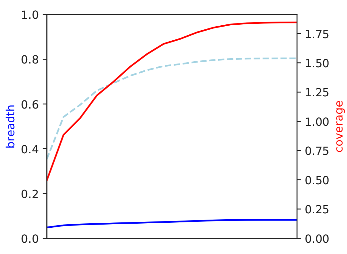
Breadth of coverage (blue line), coverage depth (red line), and expected breadth of coverage given the depth of coverage (dotted blue line) versus the minimum ANI of mapped reads. Coverage depth continues to increase while breadth of plateaus, suggesting that all regions of the reference genome are not present in the reads being mapped.

2) Genome-wide microdiversity metrics

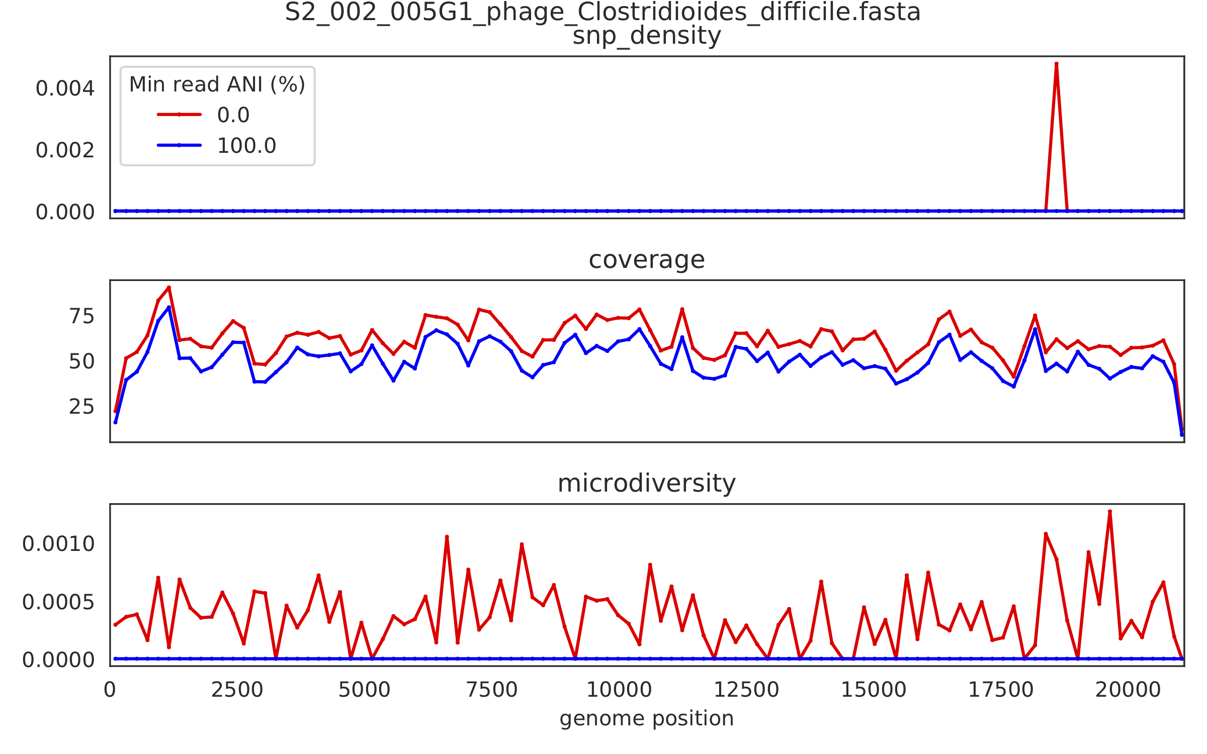
SNV density, coverage, and nucleotide diversity. Spikes in nucleotide diversity and SNV density do not correspond with increased coverage, indicating that the signals are not due to read mis-mapping. Positions with nucleotide diversity and no SNV-density are those where diversity exists but is not high enough to call a SNV

3) Read-level ANI distribution

Distribution of read pair ANI levels when mapped to a reference genome; this plot suggests that the reference genome is >1% different than the mapped reads

4) Major allele frequencies

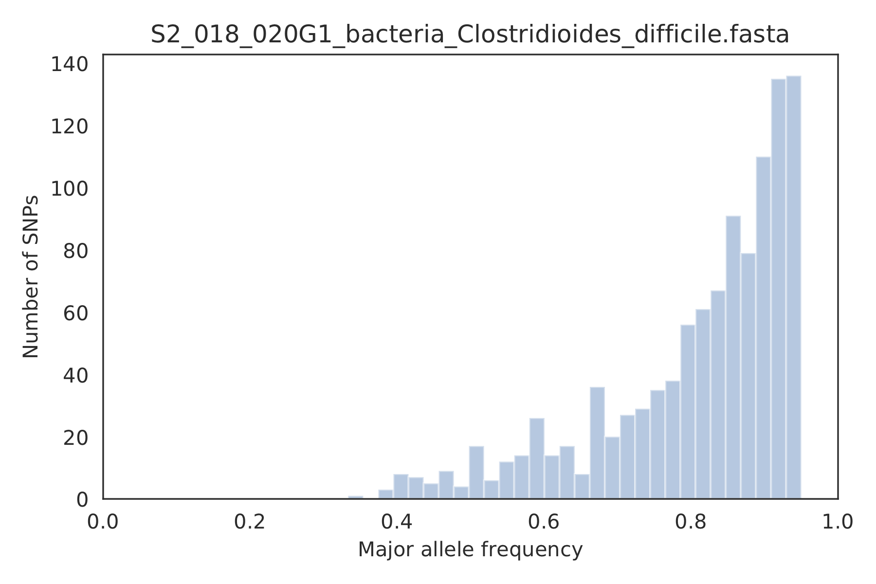
Distribution of the major allele frequencies of bi-allelic SNVs (the Site Frequency Spectrum). Alleles with major frequencies below 50% are the result of multiallelic sites. The lack of distinct puncta suggest that more than a few distinct strains are present.

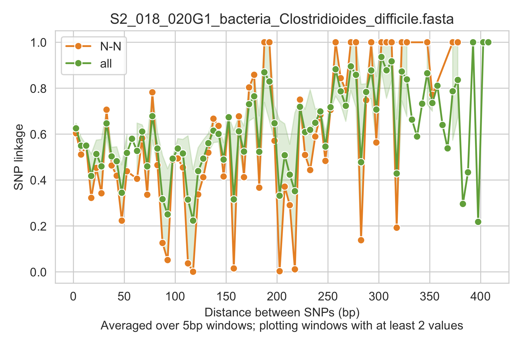
5) Linkage decay

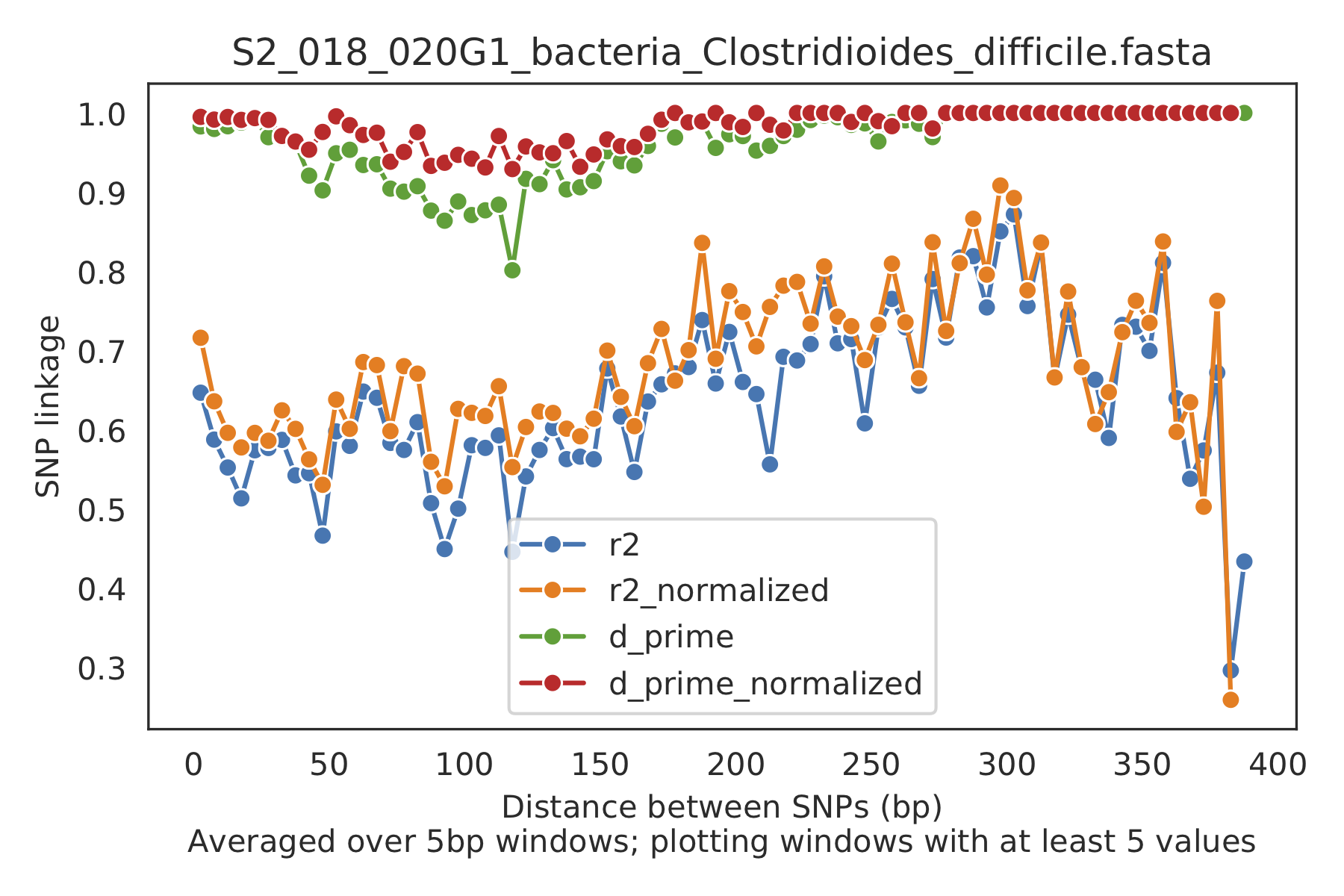
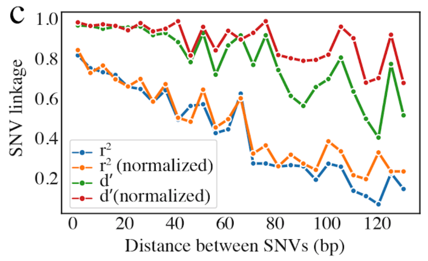
Metrics of SNV linkage vs. distance between SNVs; linkage decay (shown in one plot and not the other) is a common signal of recombination.

6) Read filtering plots

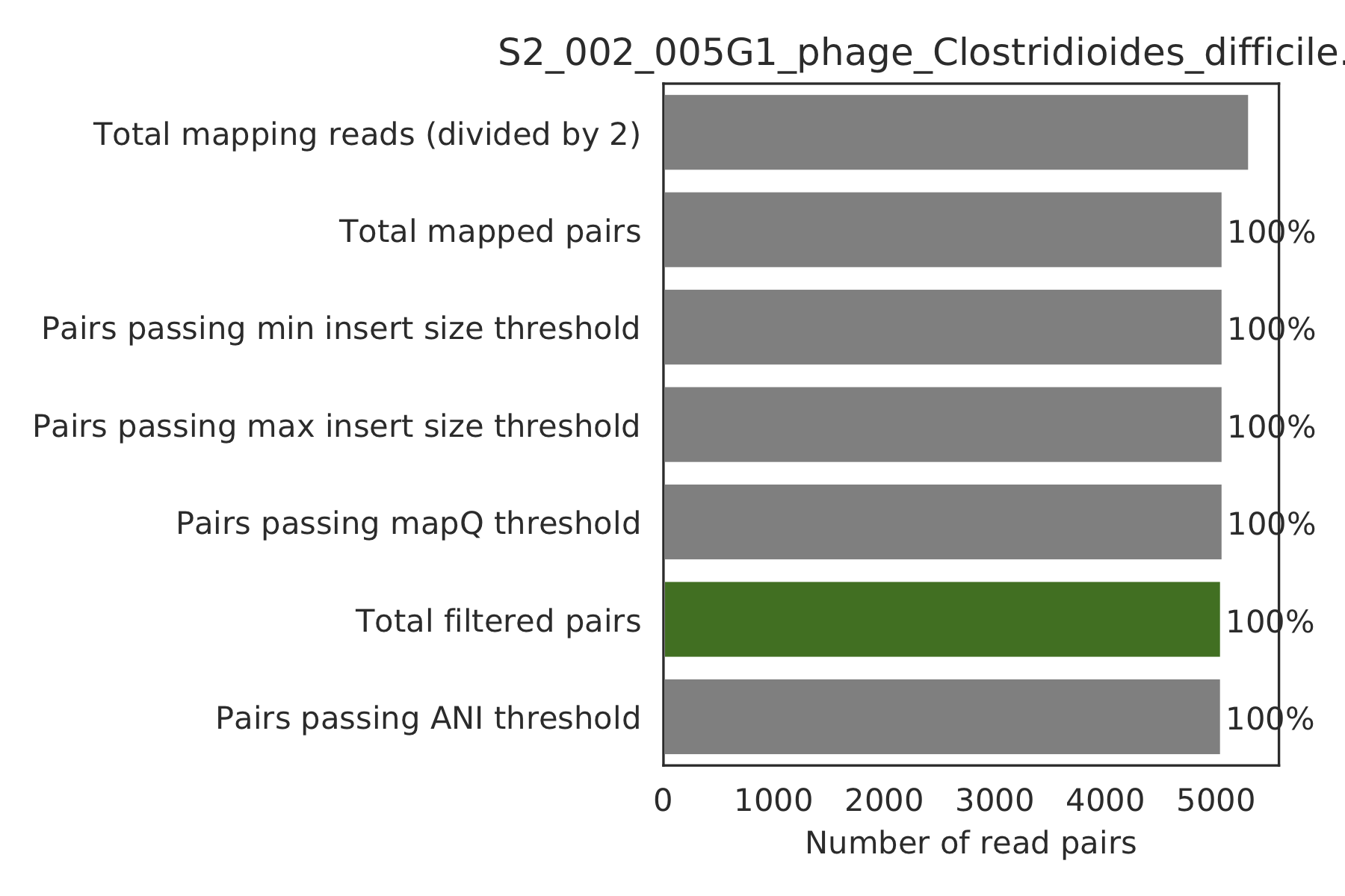
Bar plots showing how many reads got filtered out during filtering. All percentages are based on the number of paired reads; for an idea of how many reads were filtered out for being non-paired, compare the top bar and the second to top bar.

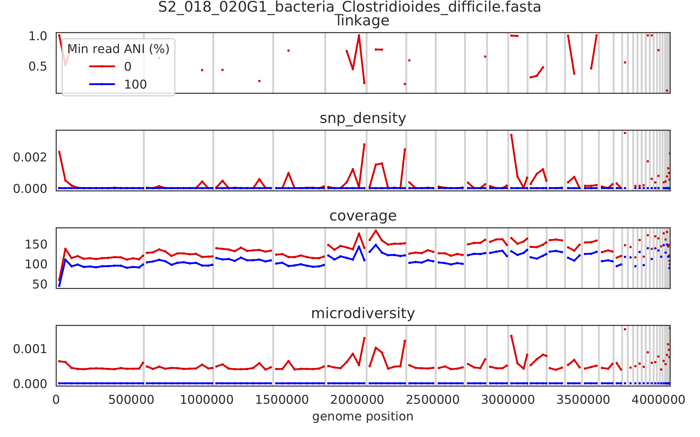
7) Scaffold inspection plot (large)

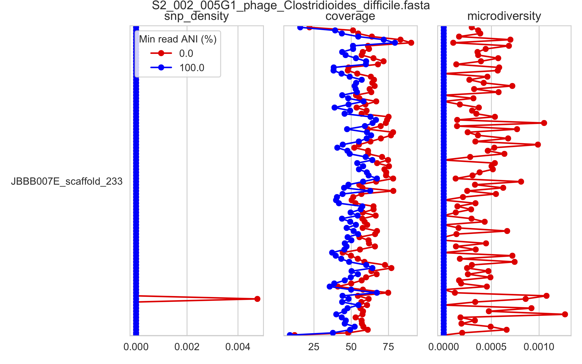
This is an elongated version of the genome-wide microdiversity metrics that is long enough for you to read scaffold names on the y-axis

8) Linkage with SNP type (GENES REQUIRED)

Linkage plot for pairs of non-synonymous SNPs and all pairs of SNPs

9) Gene histograms (GENES REQUIRED)

Histogram of values for all genes profiled

10) Compare dendrograms (RUN ON COMPARE; NOT PROFILE)

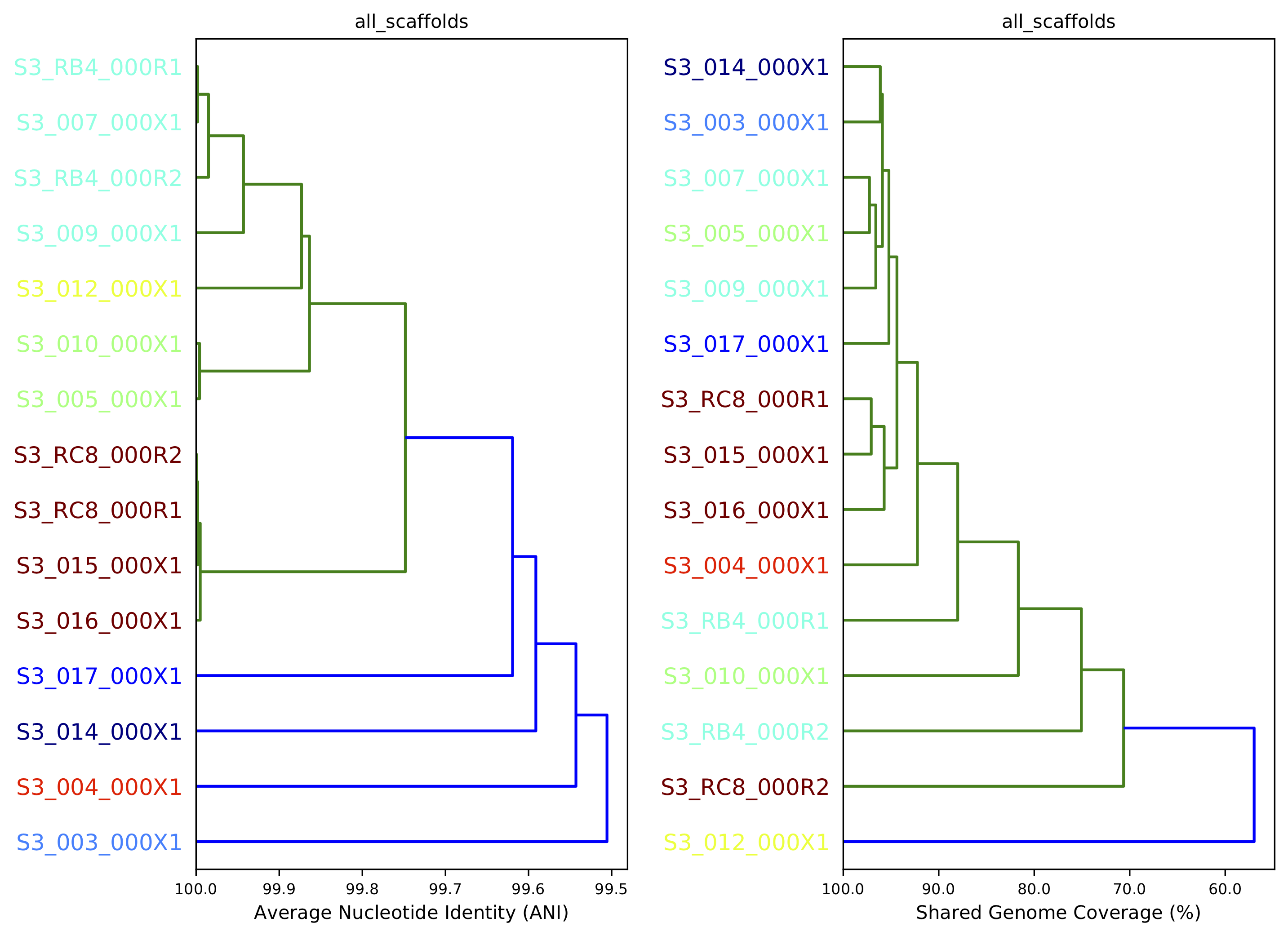
A dendrogram comparing all samples based on popANI and based on shared_bases.